World Bank Data
The World Bank is one of the world’s largest producers of development data and research. It is a great source of global socio-economic data, spanning several decades and many topics. For example, you can read their 2018 Atlas of Sustainable Development Goals or a blog post on their all-new visual guide to data and development.
The wbstats package allows you to search for and download any open World Bank dataset. To identify the actual indicator you want, you have to find its code either in the World Bank datacatalog or, even better, through wbstats.
Population Growth 1970-2017
Suppose we wanted to get data on population growth. Manually, we would navigate to the World Bank datacatalog website, and search for population growth.
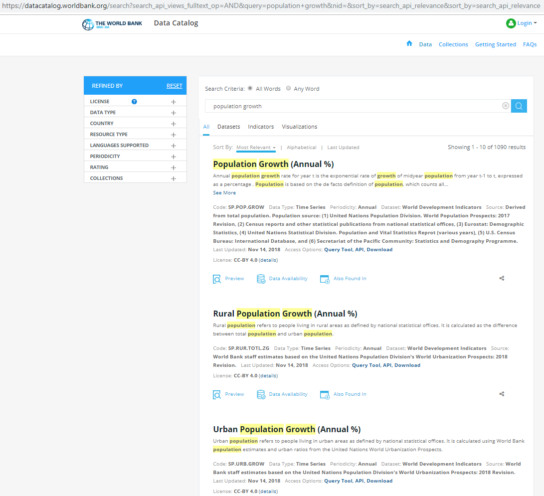
We get various results, but the more important ones are usually at the top with data on Population Growth (Annual %) with code SP.POP.GROW, on Rural Population Growth (Annual %) with code SP.RUR.TOTL.ZG, and on Urban Population Growth (Annual %) with code SP.URB.GROW.
Alternatively, we would load the wbstats package, and use pop_growth_codes <- wbsearch(pattern = "population growth") to get a dataframe with the codes that the search function returns.
library(wbstats)

pop_growth_codes <- wb_search(pattern = "population growth")
head(pop_growth_codes)
## # A tibble: 4 x 3
## indicator_id indicator indicator_desc
## <chr> <chr> <chr>
## 1 IN.EC.POP.GRWT~ Decadal Growth of P~ Population growth rate over the 10 year ~
## 2 SP.POP.GROW Population growth (~ Annual population growth rate for year t~
## 3 SP.RUR.TOTL.ZG Rural population gr~ Rural population refers to people living~
## 4 SP.URB.GROW Urban population gr~ Urban population refers to people living~Either way, the indicator we are interested in is Population Growth Annual and its code = SP.POP.GROW. The next step is to download the data with the wbstats::wb_data() function.
The first argument the wb_data function takes is a list of countries; if left empty, is will download all data for individual countries and aggregate regions like Arab World, Euro area, etc. In our example, let us download data for individuals countries only starting at 1970 and ending in 2017.
# Download data for Population Growth Annual% SP.POP.GROW
pop_growth_data <- wb_data(country = "countries_only",
                      indicator = "SP.POP.GROW",
                      start_date = 1970,
                      end_date = 2017,
                      return_wide=FALSE)

glimpse(pop_growth_data)
## Rows: 10,416
## Columns: 11
## $ indicator_id <chr> "SP.POP.GROW", "SP.POP.GROW", "SP.POP.GROW", "SP.POP.G...
## $ indicator <chr> "Population growth (annual %)", "Population growth (an...
## $ iso2c <chr> "AF", "AF", "AF", "AF", "AF", "AF", "AF", "AF", "AF", ...
## $ iso3c <chr> "AFG", "AFG", "AFG", "AFG", "AFG", "AFG", "AFG", "AFG"...
## $ country <chr> "Afghanistan", "Afghanistan", "Afghanistan", "Afghanis...
## $ date <dbl> 2017, 2016, 2015, 2014, 2013, 2012, 2011, 2010, 2009, ...
## $ value <dbl> 2.55, 2.78, 3.08, 3.36, 3.49, 3.41, 3.14, 2.75, 2.40, ...
## $ unit <chr> NA, NA, NA, NA, NA, NA, NA, NA, NA, NA, NA, NA, NA, NA...
## $ obs_status <chr> NA, NA, NA, NA, NA, NA, NA, NA, NA, NA, NA, NA, NA, NA...
## $ footnote <chr> NA, NA, NA, NA, NA, NA, NA, NA, NA, NA, NA, NA, NA, NA...
## $ last_updated <date> 2020-08-18, 2020-08-18, 2020-08-18, 2020-08-18, 2020-...The wb_cachelist is a cached version of useful information from the World Bank API and provides a snapshot of available countries, indicators, and other relevant information. The structure of wb_cachelist is as follows
glimpse(wb_cachelist, max.level = 1)## List of 8
## $ countries : tibble [304 x 18] (S3: tbl_df/tbl/data.frame)
## $ indicators : tibble [16,607 x 8] (S3: tbl_df/tbl/data.frame)
## $ sources : tibble [61 x 9] (S3: tbl_df/tbl/data.frame)
## $ topics : tibble [21 x 3] (S3: tbl_df/tbl/data.frame)
## $ regions : tibble [48 x 4] (S3: tbl_df/tbl/data.frame)
## $ income_levels: tibble [7 x 3] (S3: tbl_df/tbl/data.frame)
## $ lending_types: tibble [4 x 3] (S3: tbl_df/tbl/data.frame)
## $ languages : tibble [23 x 3] (S3: tbl_df/tbl/data.frame)and as we can see it contains data on countries and aggregate regions, well over 16,000 indicators, etc. If we wanted to see the data on countries, let us create a dataframecountries` and glimpse its contents.
countries <-  wb_cachelist$countries
glimpse(countries)
## Rows: 304
## Columns: 18
## $ iso3c <chr> "ABW", "AFG", "AFR", "AGO", "ALB", "AND", "ANR",...
## $ iso2c <chr> "AW", "AF", "A9", "AO", "AL", "AD", "L5", "1A", ...
## $ country <chr> "Aruba", "Afghanistan", "Africa", "Angola", "Alb...
## $ capital_city <chr> "Oranjestad", "Kabul", NA, "Luanda", "Tirane", "...
## $ longitude <dbl> -70.02, 69.18, NA, 13.24, 19.82, 1.52, NA, NA, 5...
## $ latitude <dbl> 12.52, 34.52, NA, -8.81, 41.33, 42.51, NA, NA, 2...
## $ region_iso3c <chr> "LCN", "SAS", NA, "SSF", "ECS", "ECS", NA, NA, "...
## $ region_iso2c <chr> "ZJ", "8S", NA, "ZG", "Z7", "Z7", NA, NA, "ZQ", ...
## $ region <chr> "Latin America & Caribbean", "South Asia", "Aggr...
## $ admin_region_iso3c <chr> NA, "SAS", NA, "SSA", "ECA", NA, NA, NA, NA, "LA...
## $ admin_region_iso2c <chr> NA, "8S", NA, "ZF", "7E", NA, NA, NA, NA, "XJ", ...
## $ admin_region <chr> NA, "South Asia", NA, "Sub-Saharan Africa (exclu...
## $ income_level_iso3c <chr> "HIC", "LIC", NA, "LMC", "UMC", "HIC", NA, NA, "...
## $ income_level_iso2c <chr> "XD", "XM", NA, "XN", "XT", "XD", NA, NA, "XD", ...
## $ income_level <chr> "High income", "Low income", "Aggregates", "Lowe...
## $ lending_type_iso3c <chr> "LNX", "IDX", NA, "IBD", "IBD", "LNX", NA, NA, "...
## $ lending_type_iso2c <chr> "XX", "XI", NA, "XF", "XF", "XX", NA, NA, "XX", ...
## $ lending_type <chr> "Not classified", "IDA", "Aggregates", "IBRD", "...The dataframe contains the ISO country codes, the country name, its capital with its longitude and latitude, the region the country is in, the regions associated ISO code, as well as a classification on the income group, the country’s classification by income level, etc.
We can merge the dataframes pop_growth_data and countries with a left join, so we have a dataframe that contains data from both of them
countries <-  wb_cachelist$countries


# Merge with a left_join (a) country data with (b) population growth data
pop_growth <-
  left_join(countries, pop_growth_data, by="iso3c") %>%
              mutate(year = as.integer(date)) %>%  #make year an integer, rather than a character value
              select(iso3c, country.x, region, income_level, value, year=) %>%
              na.omit()
Let us calculate and plot the average population growth for all countries between 1970 and 2017, faceted by region.
average_pop_growth <- pop_growth %>%
              dplyr::group_by(region, income_level, country.x, iso3c) %>%
              summarise(average_growth = mean(value)) %>%
              arrange(average_growth) %>%
              ungroup()

ggplot(data = average_pop_growth,
       aes(x = reorder(country.x, average_growth),
           y = average_growth,
           fill = region))+
  geom_col()+
  coord_flip()+
  theme_minimal(7)+
  expand_limits(y=c(-1,8))+
  facet_wrap(~income_level, nrow=3, scales="free")+
  labs(title = 'Average annual population growth (%), 1970-2017',
       x = "",
       y = "Average Annual Population Growth (in %)",
       caption = 'Source: Worldbank') +
  # theme(legend.position="none")+
  NULL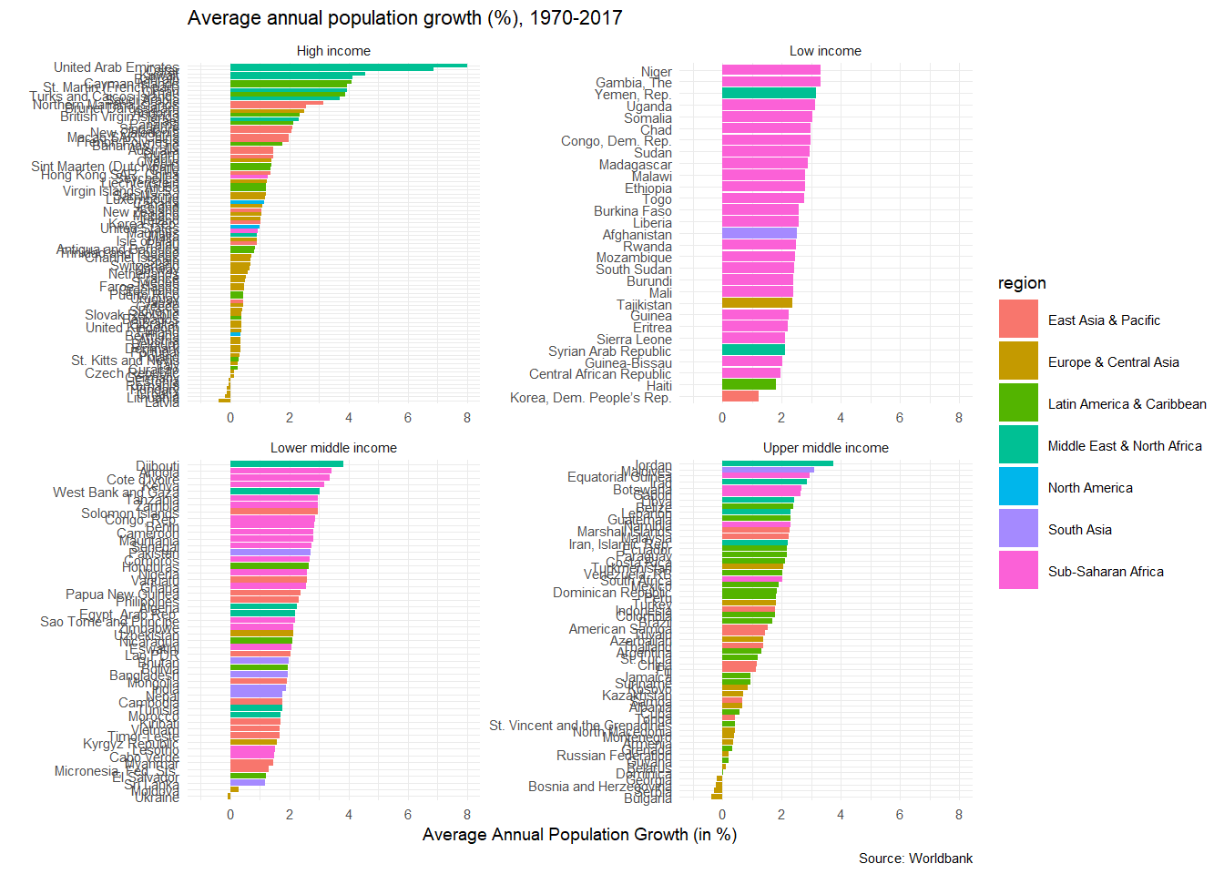
World Happiness: how does it correlate with various indicators
Data from the UN’s World Happiness Report is available at Kaggle. We have downloaded the 2015 report in a CSV file, and have a quick glimpse at its structure.
world_happiness_2015 <- read_csv(here::here("data", "world_happiness_2015.csv"))
glimpse(world_happiness_2015)
As you notice, some of the variable names include a space, like Happiness Rank, all start with a capital letter, etc. We will use janitor::clean_names() to clean the variable names, so they are easier to deal with.
library(janitor)

world_happiness_2015 <- world_happiness_2015 %>%
  clean_names()

glimpse(world_happiness_2015)
## Rows: 158
## Columns: 12
## $ country <chr> "Switzerland", "Iceland", "Denmark", "N...
## $ region <chr> "Western Europe", "Western Europe", "We...
## $ happiness_rank <dbl> 1, 2, 3, 4, 5, 6, 7, 8, 9, 10, 11, 12, ...
## $ happiness_score <dbl> 7.59, 7.56, 7.53, 7.52, 7.43, 7.41, 7.3...
## $ standard_error <dbl> 0.0341, 0.0488, 0.0333, 0.0388, 0.0355,...
## $ economy_gdp_per_capita <dbl> 1.397, 1.302, 1.325, 1.459, 1.326, 1.29...
## $ family <dbl> 1.350, 1.402, 1.361, 1.331, 1.323, 1.31...
## $ health_life_expectancy <dbl> 0.941, 0.948, 0.875, 0.885, 0.906, 0.88...
## $ freedom <dbl> 0.666, 0.629, 0.649, 0.670, 0.633, 0.64...
## $ trust_government_corruption <dbl> 0.4198, 0.1414, 0.4836, 0.3650, 0.3296,...
## $ generosity <dbl> 0.2968, 0.4363, 0.3414, 0.3470, 0.4581,...
## $ dystopia_residual <dbl> 2.52, 2.70, 2.49, 2.47, 2.45, 2.62, 2.4...First, we can look how happiness_score correlates with its of the variables the UN uses. We will use GGally:ggpairs() to get a correlation- scatterplot matrix. We do not want to include in our analyses the country name, its region, the happiness_rank and the standard error associated with the estimate of the happiness score.
world_happiness_2015 %>%
  select(-country, -region, -happiness_rank, -standard_error) %>%
  GGally::ggpairs()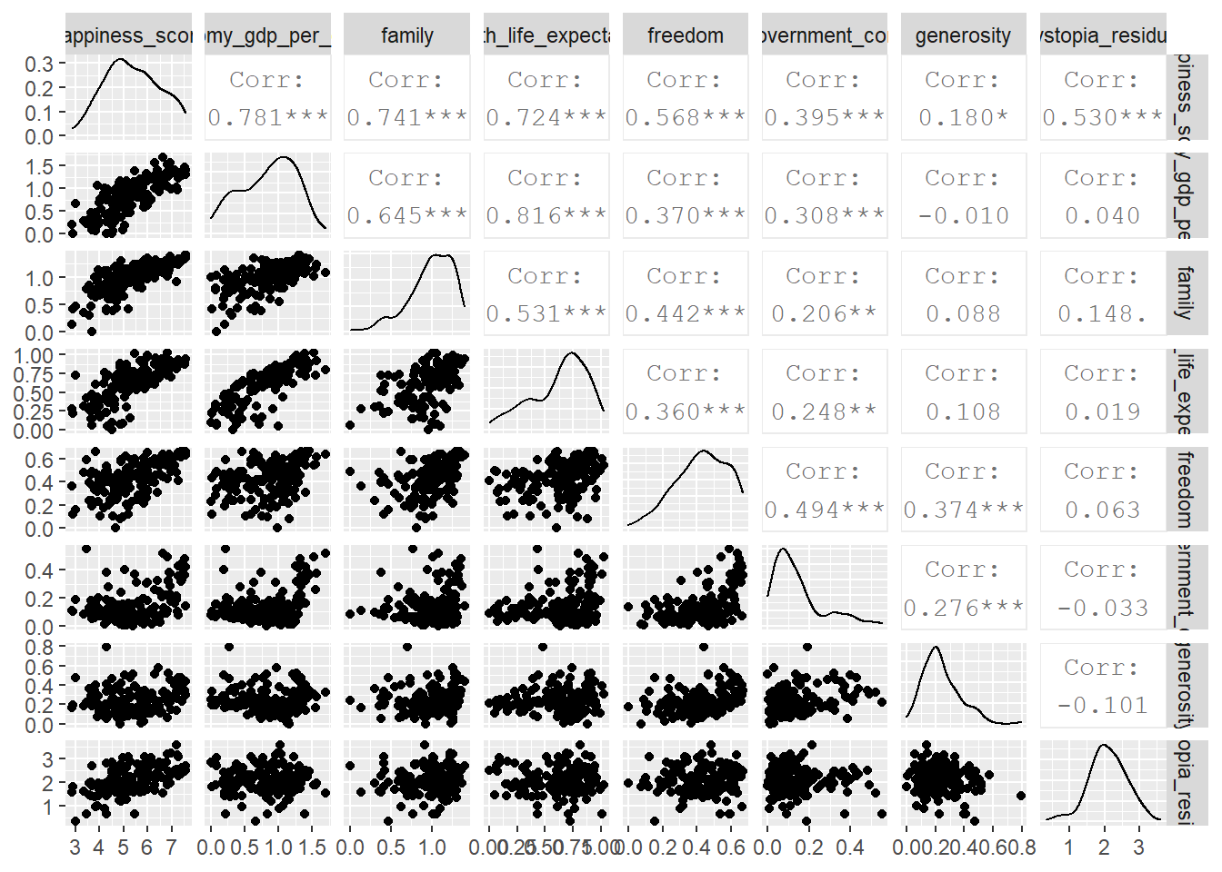
We will now choose six (6) indicators form the World Bank data, downloads their values for 2015 and see how these correlate with the overall happiness score.
# Download data for the following indicators

indicators <- c("SE.PRM.NENR",     # School enrollment, primary (% net)
                "SP.DYN.LE00.IN",  # Life expectancy
                "SI.POV.DDAY",     # Extreme poverty (% earning less than $2/day)
                "EG.ELC.ACCS.ZS",  # Access to electricity
                "SI.POV.GINI",     # GINI Index
                "NY.GDP.PCAP.KD")  # GDP per capita


happiness_data_WB_long <- wb_data(country = "countries_only",
                             indicator = indicators,
                             start_date = 2015,
                             end_date = 2015,
                             #since we have many indicators, we should get the data in long format
                             return_wide=FALSE)

# look at the long dataframe
glimpse(happiness_data_WB_long)
## Rows: 1,302
## Columns: 11
## $ indicator_id <chr> "SE.PRM.NENR", "SE.PRM.NENR", "SE.PRM.NENR", "SE.PRM.N...
## $ indicator <chr> "School enrollment, primary (% net)", "School enrollme...
## $ iso2c <chr> "AF", "AL", "DZ", "AS", "AD", "AO", "AG", "AR", "AM", ...
## $ iso3c <chr> "AFG", "ALB", "DZA", "ASM", "AND", "AGO", "ATG", "ARG"...
## $ country <chr> "Afghanistan", "Albania", "Algeria", "American Samoa",...
## $ date <dbl> 2015, 2015, 2015, 2015, 2015, 2015, 2015, 2015, 2015, ...
## $ value <dbl> NA, 94.2, 97.5, NA, NA, NA, 94.2, 99.5, 92.7, NA, 97.0...
## $ unit <chr> NA, NA, NA, NA, NA, NA, NA, NA, NA, NA, NA, NA, NA, NA...
## $ obs_status <chr> NA, NA, NA, NA, NA, NA, NA, NA, NA, NA, NA, NA, NA, NA...
## $ footnote <chr> NA, NA, NA, NA, NA, NA, NA, NA, NA, NA, NA, NA, "Natio...
## $ last_updated <date> 2020-08-18, 2020-08-18, 2020-08-18, 2020-08-18, 2020-...In order to get the two dataframes to combine into one, they have to have a shared column/ variable. We will merge the two datasets with a left_join() by “country”, and glimpse the structure of the resulting dataframe.
# Merge with a left_join (a) happiness data with all indicators and (b) the 2015 World Happiness index

happiness <-
  left_join(happiness_data_WB_long, world_happiness_2015, by="country")

glimpse(happiness)
## Rows: 1,302
## Columns: 22
## $ indicator_id <chr> "SE.PRM.NENR", "SE.PRM.NENR", "SE.PRM.N...
## $ indicator <chr> "School enrollment, primary (% net)", "...
## $ iso2c <chr> "AF", "AL", "DZ", "AS", "AD", "AO", "AG...
## $ iso3c <chr> "AFG", "ALB", "DZA", "ASM", "AND", "AGO...
## $ country <chr> "Afghanistan", "Albania", "Algeria", "A...
## $ date <dbl> 2015, 2015, 2015, 2015, 2015, 2015, 201...
## $ value <dbl> NA, 94.2, 97.5, NA, NA, NA, 94.2, 99.5,...
## $ unit <chr> NA, NA, NA, NA, NA, NA, NA, NA, NA, NA,...
## $ obs_status <chr> NA, NA, NA, NA, NA, NA, NA, NA, NA, NA,...
## $ footnote <chr> NA, NA, NA, NA, NA, NA, NA, NA, NA, NA,...
## $ last_updated <date> 2020-08-18, 2020-08-18, 2020-08-18, 20...
## $ region <chr> "Southern Asia", "Central and Eastern E...
## $ happiness_rank <dbl> 153, 95, 68, NA, NA, 137, NA, 30, 127, ...
## $ happiness_score <dbl> 3.58, 4.96, 5.61, NA, NA, 4.03, NA, 6.5...
## $ standard_error <dbl> 0.0308, 0.0501, 0.0510, NA, NA, 0.0476,...
## $ economy_gdp_per_capita <dbl> 0.320, 0.879, 0.939, NA, NA, 0.758, NA,...
## $ family <dbl> 0.303, 0.804, 1.078, NA, NA, 0.860, NA,...
## $ health_life_expectancy <dbl> 0.3034, 0.8133, 0.6177, NA, NA, 0.1668,...
## $ freedom <dbl> 0.2341, 0.3573, 0.2858, NA, NA, 0.1038,...
## $ trust_government_corruption <dbl> 0.09719, 0.06413, 0.17383, NA, NA, 0.07...
## $ generosity <dbl> 0.3651, 0.1427, 0.0782, NA, NA, 0.1234,...
## $ dystopia_residual <dbl> 1.95, 1.90, 2.43, NA, NA, 1.95, NA, 2.8...We can create a histogram of happiness_score by region
ggplot(data = happiness, aes(x = happiness_score , fill=region))+
  geom_histogram()+
  theme_minimal()+
  facet_wrap(~region,nrow=5) +
  labs(title = '2015 World Happiness',
       x = "",
       y = "Total Happiness Score",
       caption = 'Source: Worldbank') +
  theme(legend.position="none")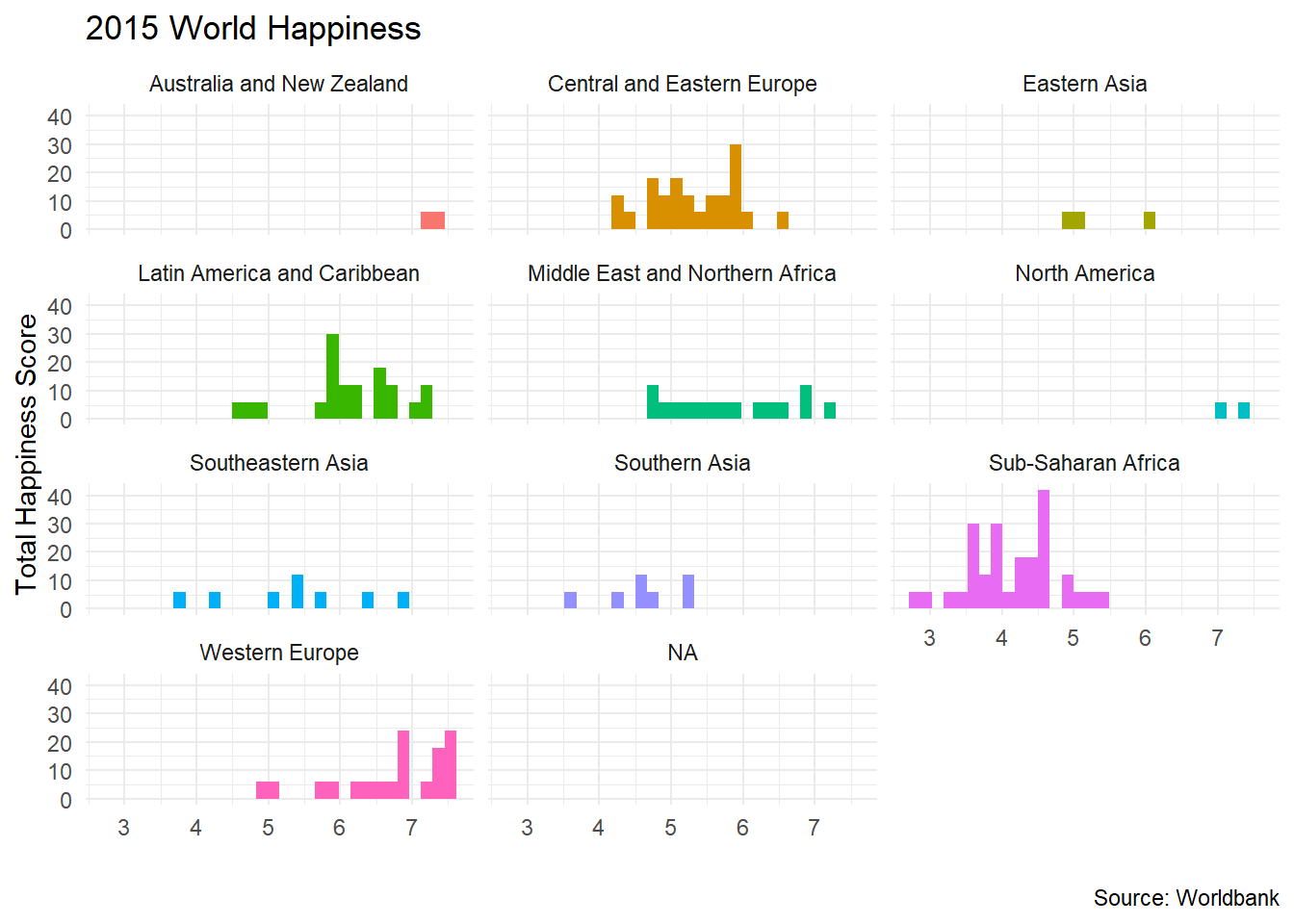
We can also create a scatterplot of happiness_score against all the indicators we have downloaded.
ggplot(data = happiness, aes(x = value, y = happiness_score , colour=indicator))+
  geom_point()+
  geom_smooth(se=FALSE)+
  theme_minimal()+
  facet_wrap(~indicator,scales="free") +
  labs(title = '2015 World Happiness',
       x = "",
       y = "Total Happiness Score",
       caption = 'Source: Worldbank') +
  theme(legend.position="none")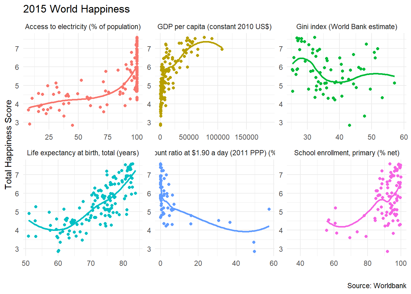
Acknowledgments
- This page is derived in part from Introduction to the
wbstatsR-package by Jesse Piburn.