Using SQL within R
SQL and dbplyr
This sort note will teach you the basics of using SQL databases with R. Sometimes, you have a massive dataset, made up of many different dataframes (or tables in SQL jargon), that would crash your computer’s memory if you try to load it. To interact with any database you typically use SQL, the Structured Query Language.
Rather than writing SQL commands, the dbplyr package automatically generates SQL commands from dplyr sequences. However, please keep in mind that SQL is a very large language, and dbplyr doesn’t do everything, but you can still get a lot out of it.
SQL commands vs dplyr verbs
One of the advantages of learning about tidy data and dplyr is that with dplyr verbs you can replicate a lot of what SQL does.
SQL command… |
… translate to dplyr verb |
|---|---|
| SELECT |
|
| FROM | which dataframe to use |
| WHERE | filter() |
| GROUP_BY | group_by() |
| ORDER_BY | arrange() |
| LIMIT | head() |
Establish a connection with the SQLite database
We will use the European Soccer Database that has more than 25,000 matches and more than 11,000 players. We first need to establish a connection with the SQL database. Unlike dataframes that we just load into memory, the size of some SQL databases prohibits loading the entire database into memory. Although this soccer database is a locally saved file, we would use a similar connection into any SQL database over the internet
# set up a connection to sqlite database
football_db <- DBI::dbConnect(
  drv = RSQLite::SQLite(),
  dbname = "database.sqlite"
)
The general code for connecting to a remote database is:
connection_to_db <- DBI::dbConnect(
  drv = [database driver, eg odbc::odbc()],
  dbname = "database_name",
  user = "User_ID",
  password = "Password",
  host = "host name", (default=local connection)
  port = "port number" (default=local connection)
)
That’s pretty much it - R now has a direct connection to the database and you can start making queries.
Database objects or tibbles?
Now, an SQL database will typically contain multiple tables. You can think of these tables as R data frames (or tibbles). What are the tables in the soccer database? We can browse the tables in the database using DBI::dbListTables()
DBI::dbListTables(football_db)## [1] "Country" "League" "Match"
## [4] "Player" "Player_Attributes" "Team"
## [7] "Team_Attributes" "sqlite_sequence"We can easily set these tables up as database objects using dplyr
countries <- dplyr::tbl(football_db, "Country")
leagues <- dplyr::tbl(football_db, "League")
matches <- dplyr::tbl(football_db, "Match")
teams <- dplyr::tbl(football_db, "Team")
team_attributes <- dplyr::tbl(football_db, "Team_Attributes")
players <- dplyr::tbl(football_db, "Player")
player_attributes <- dplyr::tbl(football_db, "Player_Attributes")
Each of these tables are SQL database objects in your R session which you can manipulate in the same way as a dataframe.
class(countries)## [1] "tbl_SQLiteConnection" "tbl_dbi" "tbl_sql"
## [4] "tbl_lazy" "tbl"When you define these tables, you are not physically downloading them, just creating a bare minimum extract to work with.
IF you wanted to handle these as normal dataframes or tibbles, you can simply pipe the database objects to as_tibble()
player_attributes_df <- player_attributes %>% as_tibble()
class(player_attributes)
## [1] "tbl_SQLiteConnection" "tbl_dbi" "tbl_sql"
## [4] "tbl_lazy" "tbl"class(player_attributes_df)## [1] "tbl_df" "tbl" "data.frame"Notice the difference between player_atributes, a database object, and player_atributes_df, a ‘regular’ dataframe/tibble.
Now that we have player attributes as a dataframe, we can handle it the usual way and, e.g., build a scatterplot/correlation matrix with ggpairs()
player_attributes_df %>%
  filter(!is.na(preferred_foot)) %>%
  select(preferred_foot, ball_control, overall_rating) %>%
  ggpairs(aes(colour=preferred_foot, alpha = 0.3))+
  scale_colour_manual(values = c("#67a9cf","#ef8a62"))+
  scale_fill_manual(values = c("#67a9cf","#ef8a62"))+
  theme_bw()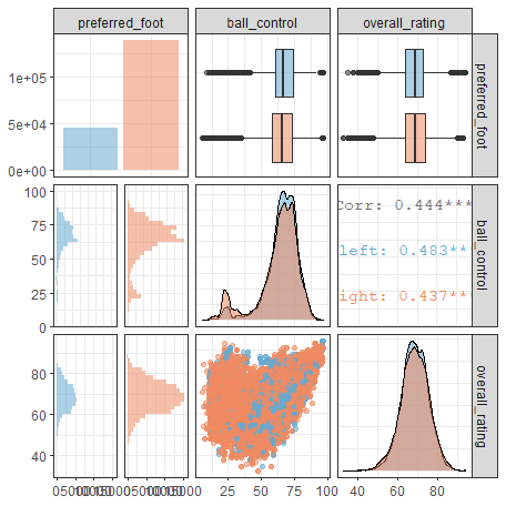
Querying the database with dbplyr
To create the ggpairs() plot we had to convert a database table to a dataframe, load it all in the computer’s memory, and then use ggplot. The beauty of working with databases is that we do NOT have to load everything into memory. Instead, all dplyr calls are evaluated lazily, generating SQL code that is only sent to the database when you request the data.
Let us look at an example. What if we wanted to calculate the average number of goals per league (country) per season and then plot those averages. This seems like a data wrangling exercise we would do with dplyr
# write dplyr code that will calculate average number of goals per country per season
goals_per_match <-  matches %>%
  group_by(country_id, season) %>%
  summarise(avg_goals = mean(home_team_goal + away_team_goal)) %>%

  #do a left_join, so we know the country's name rather than the country's ID
  left_join(countries, by = c("country_id"="id")) %>%
  arrange(desc(avg_goals)) %>%
  ungroup()
What kind of an object is goals_per_match?
#what kind of an object is goals_per_match?
class(goals_per_match)
## [1] "tbl_SQLiteConnection" "tbl_dbi" "tbl_sql"
## [4] "tbl_lazy" "tbl"goals_per_match is not a dataframe (tibble), but rather a query to an SQLite database table.
Generate the actual SQL commands
We are familiar with all the dplyr verbs (filter, select, group_by, summarise, arrange, etc.), but SQL has its own commands, all of which are written in capital letters (is SQL constantly angry and shouting? Who knew…). We can generate the actual SQL commands using dbplyr::sql_render() or dplyr::show_query()
# Generate actual SQL commands: We can either use dbplyr::sql_render() or dplyr::show_query()
dbplyr::sql_render(goals_per_match)
## <SQL> SELECT *
## FROM (SELECT `LHS`.`country_id` AS `country_id`, `LHS`.`season` AS `season`, `LHS`.`avg_goals` AS `avg_goals`, `RHS`.`name` AS `name`
## FROM (SELECT `country_id`, `season`, AVG(`home_team_goal` + `away_team_goal`) AS `avg_goals`
## FROM `Match`
## GROUP BY `country_id`, `season`) AS `LHS`
## LEFT JOIN `Country` AS `RHS`
## ON (`LHS`.`country_id` = `RHS`.`id`)
## )
## ORDER BY `avg_goals` DESCgoals_per_match %>% show_query()## <SQL>
## SELECT *
## FROM (SELECT `LHS`.`country_id` AS `country_id`, `LHS`.`season` AS `season`, `LHS`.`avg_goals` AS `avg_goals`, `RHS`.`name` AS `name`
## FROM (SELECT `country_id`, `season`, AVG(`home_team_goal` + `away_team_goal`) AS `avg_goals`
## FROM `Match`
## GROUP BY `country_id`, `season`) AS `LHS`
## LEFT JOIN `Country` AS `RHS`
## ON (`LHS`.`country_id` = `RHS`.`id`)
## )
## ORDER BY `avg_goals` DESCRun SQL query and retrieve results
Now that we have the SQL query we can retrieve the results into a local dataframe (tibble) using collect(). The main difference is that rather than loading all of the databases in memory, the goals_per_match goes to the SQL database, collects the necessary data, and only returns
# execute query and retrieve results in a tibble (dataframe).
goals_match_tibble <- goals_per_match %>%
  collect()

#have a look at the resulting dataframe with glimpse() and skim()
glimpse(goals_match_tibble)
## Rows: 88
## Columns: 4
## $ country_id <int> 24558, 13274, 13274, 13274, 7809, 13274, 24558, 13274, 2...
## $ season <chr> "2009/2010", "2011/2012", "2010/2011", "2013/2014", "201...
## $ avg_goals <dbl> 3.33, 3.26, 3.23, 3.20, 3.16, 3.15, 3.14, 3.08, 3.00, 2....
## $ name <chr> "Switzerland", "Netherlands", "Netherlands", "Netherland...skimr::skim(goals_match_tibble)| Name | goals_match_tibble |
| Number of rows | 88 |
| Number of columns | 4 |
| _______________________ | |
| Column type frequency: | |
| character | 2 |
| numeric | 2 |
| ________________________ | |
| Group variables | None |
Variable type: character
| skim_variable | n_missing | complete_rate | min | max | empty | n_unique | whitespace |
|---|---|---|---|---|---|---|---|
| season | 0 | 1 | 9 | 9 | 0 | 8 | 0 |
| name | 0 | 1 | 5 | 11 | 0 | 11 | 0 |
Variable type: numeric
| skim_variable | n_missing | complete_rate | mean | sd | p0 | p25 | p50 | p75 | p100 | hist |
|---|---|---|---|---|---|---|---|---|---|---|
| country_id | 0 | 1 | 12452.09 | 7877.88 | 1.00 | 4769.00 | 13274.00 | 19694.00 | 24558.00 | ▇▂▅▅▇ |
| avg_goals | 0 | 1 | 2.71 | 0.24 | 2.18 | 2.56 | 2.71 | 2.86 | 3.33 | ▂▆▇▃▂ |
The resulting dataframe only has the information we want: 4 variables (columns) and 88 rows (cases); for each country and season, we have the average number of goals scored per match. We can now use this smaller dataframe and plot the results.
# plot results, using goals_match_tibble
ggplot(goals_match_tibble) +
  geom_point(aes(x=reorder(name, avg_goals),y=avg_goals, colour=name))+
  theme_bw(8)+
  facet_wrap(~season, nrow=4)+
  labs(
    title = "Which football leagues had the higest number of goals per game?",
    y = "Average Number of Goals per Match",
   x = "National League"
    ) +
  coord_flip() +
  theme(legend.position = "none")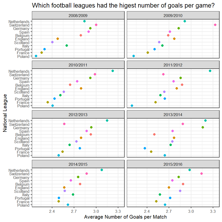
ggplot(goals_match_tibble, aes(x=reorder(name, avg_goals),y=avg_goals, colour=name)) +
  geom_violin()+
  # geom_boxplot()+
  geom_jitter()+
  theme_bw()+
  labs(
    title = "Which football leagues had the higest number of goals per game?",
    subtitle="2008/2009 to 2015/2016",
    y = "Average Number of Goals per Match",
    x = "National League"
  ) +
  coord_flip() +
  theme(legend.position = "none")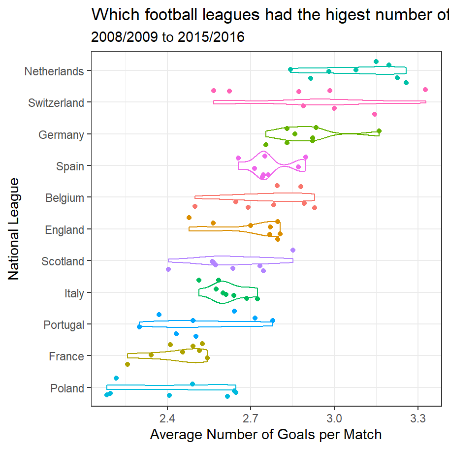
We can now run queries on the database, collect the results in a local dataframe, and show the results of, e.g., the highest overall rating of all players in the database.
# Which are the top 20 players by overall rating (`overall_rating`)?
top_players <-  player_attributes %>%
  group_by(player_api_id) %>%
  summarise(max_rating = max(overall_rating)) %>%
  arrange(desc(max_rating)) %>%
  left_join(players, by = c("player_api_id"="player_api_id")) %>%
  collect

top_players %>%
  head(20) %>%
kableExtra::kable()| player_api_id | max_rating | id | player_name | player_fifa_api_id | birthday | height | weight |
|---|---|---|---|---|---|---|---|
| 30981 | 94 | 6176 | Lionel Messi | 158023 | 1987-06-24 00:00:00 | 170 | 159 |
| 30893 | 93 | 1995 | Cristiano Ronaldo | 20801 | 1985-02-05 00:00:00 | 185 | 176 |
| 30829 | 93 | 10749 | Wayne Rooney | 54050 | 1985-10-24 00:00:00 | 175 | 183 |
| 30717 | 93 | 3826 | Gianluigi Buffon | 1179 | 1978-01-28 00:00:00 | 193 | 201 |
| 39989 | 92 | 3994 | Gregory Coupet | 1747 | 1972-12-31 00:00:00 | 180 | 176 |
| 39854 | 92 | 10861 | Xavi Hernandez | 10535 | 1980-01-25 00:00:00 | 170 | 148 |
| 34520 | 91 | 3183 | Fabio Cannavaro | 1183 | 1973-09-13 00:00:00 | 175 | 165 |
| 30955 | 91 | 742 | Andres Iniesta | 41 | 1984-05-11 00:00:00 | 170 | 150 |
| 30743 | 91 | 9216 | Ronaldinho | 28130 | 1980-03-21 00:00:00 | 183 | 168 |
| 30723 | 91 | 388 | Alessandro Nesta | 1088 | 1976-03-19 00:00:00 | 188 | 174 |
| 30657 | 91 | 4366 | Iker Casillas | 5479 | 1981-05-20 00:00:00 | 185 | 185 |
| 30627 | 91 | 5120 | John Terry | 13732 | 1980-12-07 00:00:00 | 188 | 198 |
| 30626 | 91 | 10203 | Thierry Henry | 1625 | 1977-08-17 00:00:00 | 188 | 183 |
| 41044 | 90 | 5592 | Kaka | 138449 | 1982-04-22 00:00:00 | 185 | 183 |
| 40636 | 90 | 6377 | Luis Suarez | 176580 | 1987-01-24 00:00:00 | 183 | 187 |
| 38843 | 90 | 11039 | Ze Roberto | 28765 | 1974-07-06 00:00:00 | 173 | 159 |
| 35724 | 90 | 11057 | Zlatan Ibrahimovic | 41236 | 1981-10-03 00:00:00 | 196 | 209 |
| 30924 | 90 | 3514 | Franck Ribery | 156616 | 1983-04-07 00:00:00 | 170 | 159 |
| 30834 | 90 | 951 | Arjen Robben | 9014 | 1984-01-23 00:00:00 | 180 | 176 |
| 30728 | 90 | 2426 | David Trezeguet | 5984 | 1977-10-15 00:00:00 | 190 | 176 |
# Which are the top 20 goalkeepers by sum of all gk attributes (`gk_diving`,`gk_handling`, `gk_kicking`, etc)?
top_goalies <-  player_attributes %>%
  mutate(goalie_rating = gk_diving + gk_handling + gk_kicking + gk_positioning + gk_reflexes) %>%
  group_by(player_api_id) %>%
  summarise(max_goalie_rating = max(goalie_rating)) %>%
  arrange(desc(max_goalie_rating)) %>%
  left_join(players, by = c("player_api_id"="player_api_id")) %>%
  collect


top_goalies %>%
  head(20) %>%
kableExtra::kable()| player_api_id | max_goalie_rating | id | player_name | player_fifa_api_id | birthday | height | weight |
|---|---|---|---|---|---|---|---|
| 30717 | 449 | 3826 | Gianluigi Buffon | 1179 | 1978-01-28 00:00:00 | 193 | 201 |
| 39989 | 447 | 3994 | Gregory Coupet | 1747 | 1972-12-31 00:00:00 | 180 | 176 |
| 30859 | 445 | 8580 | Petr Cech | 48940 | 1982-05-20 00:00:00 | 196 | 198 |
| 30657 | 442 | 4366 | Iker Casillas | 5479 | 1981-05-20 00:00:00 | 185 | 185 |
| 27299 | 440 | 6556 | Manuel Neuer | 167495 | 1986-03-27 00:00:00 | 193 | 203 |
| 30989 | 438 | 5536 | Julio Cesar | 48717 | 1979-09-03 00:00:00 | 185 | 174 |
| 24503 | 437 | 9579 | Sebastian Frey | 1289 | 1980-03-18 00:00:00 | 190 | 198 |
| 30726 | 436 | 2900 | Edwin van der Sar | 51539 | 1970-10-29 00:00:00 | 198 | 196 |
| 182917 | 429 | 2340 | David De Gea | 193080 | 1990-11-07 00:00:00 | 193 | 181 |
| 30660 | 428 | 8541 | Pepe Reina | 24630 | 1982-08-31 00:00:00 | 188 | 203 |
| 30622 | 426 | 8413 | Paul Robinson | 13914 | 1979-10-15 00:00:00 | 193 | 198 |
| 32657 | 425 | 10625 | Victor Valdes | 106573 | 1982-01-14 00:00:00 | 183 | 172 |
| 30742 | 425 | 7470 | Mickael Landreau | 3813 | 1979-05-14 00:00:00 | 183 | 185 |
| 26295 | 425 | 4272 | Hugo Lloris | 167948 | 1986-12-26 00:00:00 | 188 | 172 |
| 30841 | 424 | 6446 | Maarten Stekelenburg | 2147 | 1982-09-22 00:00:00 | 198 | 203 |
| 27341 | 424 | 9028 | Robert Enke,30 | 158400 | 1977-08-24 00:00:00 | 185 | 172 |
| 30648 | 423 | 4832 | Jens Lehmann | 805 | 1969-11-10 00:00:00 | 190 | 192 |
| 33986 | 421 | 746 | Andres Palop | 8247 | 1973-10-22 00:00:00 | 183 | 165 |
| 31293 | 421 | 10009 | Steve Mandanda | 163705 | 1985-03-28 00:00:00 | 185 | 181 |
| 30380 | 420 | 1345 | Brad Friedel | 11983 | 1971-05-18 00:00:00 | 188 | 203 |