Eurostat Data
Eurostat Data with the eurostat package
The eurostat package provides access to well over 9000 datasets from the Eurostat. It may seem a challenging task to find the correct dataset, but you are essentially looking for the code that describes the dataset. We an get a table of contents, namely all of the codes contained in the eurostat database.
library(eurostat)
library(fpp2) # for time series decomposition
library(seasonal)
library(tmap) #mapping eurostat data

# Get Eurostat data listing
# Function get_eurostat_toc() downloads a table of contents of eurostat datasets.
# The values in column ‘code’ should be used to download a selected dataset.
toc <- get_eurostat_toc()

# Check the first 20 rows
head(toc, 20) %>%
kable()| title | code | type | last update of data | last table structure change | data start | data end | values |
|---|---|---|---|---|---|---|---|
| Database by themes | data | folder | NA | NA | NA | NA | NA |
| General and regional statistics | general | folder | NA | NA | NA | NA | NA |
| European and national indicators for short-term analysis | euroind | folder | NA | NA | NA | NA | NA |
| Business and consumer surveys (source: DG ECFIN) | ei_bcs | folder | NA | NA | NA | NA | NA |
| Consumer surveys (source: DG ECFIN) | ei_bcs_cs | folder | NA | NA | NA | NA | NA |
| Consumers - monthly data | ei_bsco_m | dataset | 28.05.2021 | 28.05.2021 | 1980M01 | 2021M05 | NA |
| Consumers - quarterly data | ei_bsco_q | dataset | 28.05.2021 | 29.04.2021 | 1990Q1 | 2021Q2 | NA |
| Business surveys - NACE Rev. 2 activity (source: DG ECFIN) | ei_bcs_bs | folder | NA | NA | NA | NA | NA |
| Industry - monthly data | ei_bsin_m_r2 | dataset | 28.05.2021 | 28.05.2021 | 1980M01 | 2021M05 | NA |
| Industry - quarterly data | ei_bsin_q_r2 | dataset | 28.05.2021 | 29.04.2021 | 1980Q1 | 2021Q2 | NA |
| Construction - monthly data | ei_bsbu_m_r2 | dataset | 28.05.2021 | 03.06.2021 | 1980M01 | 2021M05 | NA |
| Construction - quarterly data | ei_bsbu_q_r2 | dataset | 28.05.2021 | 29.04.2021 | 1981Q1 | 2021Q2 | NA |
| Retail sale - monthly data | ei_bsrt_m_r2 | dataset | 28.05.2021 | 28.05.2021 | 1984M01 | 2021M05 | NA |
| Sentiment indicators - monthly data | ei_bssi_m_r2 | dataset | 28.05.2021 | 18.06.2021 | 1980M01 | 2021M05 | NA |
| Services - monthly data | ei_bsse_m_r2 | dataset | 28.05.2021 | 18.06.2021 | 1988M01 | 2021M05 | NA |
| Services - quarterly data | ei_bsse_q_r2 | dataset | 28.05.2021 | 29.04.2021 | 2001Q2 | 2021Q2 | NA |
| Euro-zone Business Climate Indicator - monthly data | ei_bsci_m_r2 | dataset | 28.05.2021 | 28.05.2021 | 1985M01 | 2021M05 | NA |
| Financial services - monthly data | ei_bsfs_m | dataset | 28.05.2021 | 03.06.2021 | 2006M04 | 2021M05 | NA |
| Financial services - quarterly data | ei_bsfs_q | dataset | 28.05.2021 | 03.06.2021 | 2007Q3 | 2021Q2 | NA |
| Employment expectations indicator | ei_bsee_m_r2 | dataset | 28.05.2021 | 28.05.2021 | 1980M01 | 2021M05 | NA |
House Price Index (HPI)
The Eurostat House Price Index (HPI) measures price changes of all residential properties purchased by households (flats, detached houses, terraced houses, etc.), both new and existing, independently of their final use and their previous owners. First, we node that the code id for this dataset is teicp270. Once we know the relevant code id, we can download eurostat data using the get_eurostat(id) function.
hpi <- get_eurostat(id="teicp270")
glimpse(hpi)
## Rows: 1,256
## Columns: 5
## $ indic <chr> "TOTAL", "TOTAL", "TOTAL", "TOTAL", "TOTAL", "TOTAL", "TOTAL", ~
## $ unit <chr> "I15_NSA", "I15_NSA", "I15_NSA", "I15_NSA", "I15_NSA", "I15_NSA~
## $ geo <chr> "AT", "BE", "BG", "CY", "CZ", "DE", "DK", "EA", "EA19", "EE", "~
## $ time <date> 2018-01-01, 2018-01-01, 2018-01-01, 2018-01-01, 2018-01-01, 20~
## $ values <dbl> 117.5, 107.7, 120.7, 103.1, 125.0, 118.3, 114.0, 111.3, 111.3, ~head(hpi,40) %>%
kable()| indic | unit | geo | time | values |
|---|---|---|---|---|
| TOTAL | I15_NSA | AT | 2018-01-01 | 117.5 |
| TOTAL | I15_NSA | BE | 2018-01-01 | 107.7 |
| TOTAL | I15_NSA | BG | 2018-01-01 | 120.7 |
| TOTAL | I15_NSA | CY | 2018-01-01 | 103.1 |
| TOTAL | I15_NSA | CZ | 2018-01-01 | 125.0 |
| TOTAL | I15_NSA | DE | 2018-01-01 | 118.3 |
| TOTAL | I15_NSA | DK | 2018-01-01 | 114.0 |
| TOTAL | I15_NSA | EA | 2018-01-01 | 111.3 |
| TOTAL | I15_NSA | EA19 | 2018-01-01 | 111.3 |
| TOTAL | I15_NSA | EE | 2018-01-01 | 115.2 |
| TOTAL | I15_NSA | ES | 2018-01-01 | 115.0 |
| TOTAL | I15_NSA | EU | 2018-01-01 | 112.4 |
| TOTAL | I15_NSA | EU27_2020 | 2018-01-01 | 112.2 |
| TOTAL | I15_NSA | EU28 | 2018-01-01 | 112.4 |
| TOTAL | I15_NSA | FI | 2018-01-01 | 102.7 |
| TOTAL | I15_NSA | FR | 2018-01-01 | 105.4 |
| TOTAL | I15_NSA | HR | 2018-01-01 | 109.4 |
| TOTAL | I15_NSA | HU | 2018-01-01 | 138.7 |
| TOTAL | I15_NSA | IE | 2018-01-01 | 127.3 |
| TOTAL | I15_NSA | IS | 2018-01-01 | 138.8 |
| TOTAL | I15_NSA | IT | 2018-01-01 | 98.6 |
| TOTAL | I15_NSA | LT | 2018-01-01 | 119.8 |
| TOTAL | I15_NSA | LU | 2018-01-01 | 116.8 |
| TOTAL | I15_NSA | LV | 2018-01-01 | 126.0 |
| TOTAL | I15_NSA | MT | 2018-01-01 | 111.2 |
| TOTAL | I15_NSA | NL | 2018-01-01 | 119.9 |
| TOTAL | I15_NSA | NO | 2018-01-01 | 113.6 |
| TOTAL | I15_NSA | PL | 2018-01-01 | 109.5 |
| TOTAL | I15_NSA | PT | 2018-01-01 | 125.6 |
| TOTAL | I15_NSA | RO | 2018-01-01 | 116.1 |
| TOTAL | I15_NSA | SE | 2018-01-01 | 113.2 |
| TOTAL | I15_NSA | SI | 2018-01-01 | 118.0 |
| TOTAL | I15_NSA | SK | 2018-01-01 | 119.6 |
| TOTAL | I15_NSA | TR | 2018-01-01 | 130.9 |
| TOTAL | I15_NSA | UK | 2018-01-01 | 113.6 |
| TOTAL | PCH_Q1_NSA | AT | 2018-01-01 | 0.8 |
| TOTAL | PCH_Q1_NSA | BE | 2018-01-01 | 0.0 |
| TOTAL | PCH_Q1_NSA | BG | 2018-01-01 | 0.9 |
| TOTAL | PCH_Q1_NSA | CY | 2018-01-01 | -2.0 |
| TOTAL | PCH_Q1_NSA | CZ | 2018-01-01 | 2.2 |
Typically, the downloaded data has codes and abbreviations for all of the variables, but we can use label_eurostat to get a more verbose description.
house_price_index_data <-  hpi %>%
  label_eurostat()

head(house_price_index_data,40) %>%
kable()| indic | unit | geo | time | values |
|---|---|---|---|---|
| Total | Index, 2015=100 (NSA) | Austria | 2018-01-01 | 117.5 |
| Total | Index, 2015=100 (NSA) | Belgium | 2018-01-01 | 107.7 |
| Total | Index, 2015=100 (NSA) | Bulgaria | 2018-01-01 | 120.7 |
| Total | Index, 2015=100 (NSA) | Cyprus | 2018-01-01 | 103.1 |
| Total | Index, 2015=100 (NSA) | Czechia | 2018-01-01 | 125.0 |
| Total | Index, 2015=100 (NSA) | Germany (until 1990 former territory of the FRG) | 2018-01-01 | 118.3 |
| Total | Index, 2015=100 (NSA) | Denmark | 2018-01-01 | 114.0 |
| Total | Index, 2015=100 (NSA) | Euro area (EA11-1999, EA12-2001, EA13-2007, EA15-2008, EA16-2009, EA17-2011, EA18-2014, EA19-2015) | 2018-01-01 | 111.3 |
| Total | Index, 2015=100 (NSA) | Euro area - 19 countries (from 2015) | 2018-01-01 | 111.3 |
| Total | Index, 2015=100 (NSA) | Estonia | 2018-01-01 | 115.2 |
| Total | Index, 2015=100 (NSA) | Spain | 2018-01-01 | 115.0 |
| Total | Index, 2015=100 (NSA) | European Union (EU6-1958, EU9-1973, EU10-1981, EU12-1986, EU15-1995, EU25-2004, EU27-2007, EU28-2013, EU27-2020) | 2018-01-01 | 112.4 |
| Total | Index, 2015=100 (NSA) | European Union - 27 countries (from 2020) | 2018-01-01 | 112.2 |
| Total | Index, 2015=100 (NSA) | European Union - 28 countries (2013-2020) | 2018-01-01 | 112.4 |
| Total | Index, 2015=100 (NSA) | Finland | 2018-01-01 | 102.7 |
| Total | Index, 2015=100 (NSA) | France | 2018-01-01 | 105.4 |
| Total | Index, 2015=100 (NSA) | Croatia | 2018-01-01 | 109.4 |
| Total | Index, 2015=100 (NSA) | Hungary | 2018-01-01 | 138.7 |
| Total | Index, 2015=100 (NSA) | Ireland | 2018-01-01 | 127.3 |
| Total | Index, 2015=100 (NSA) | Iceland | 2018-01-01 | 138.8 |
| Total | Index, 2015=100 (NSA) | Italy | 2018-01-01 | 98.6 |
| Total | Index, 2015=100 (NSA) | Lithuania | 2018-01-01 | 119.8 |
| Total | Index, 2015=100 (NSA) | Luxembourg | 2018-01-01 | 116.8 |
| Total | Index, 2015=100 (NSA) | Latvia | 2018-01-01 | 126.0 |
| Total | Index, 2015=100 (NSA) | Malta | 2018-01-01 | 111.2 |
| Total | Index, 2015=100 (NSA) | Netherlands | 2018-01-01 | 119.9 |
| Total | Index, 2015=100 (NSA) | Norway | 2018-01-01 | 113.6 |
| Total | Index, 2015=100 (NSA) | Poland | 2018-01-01 | 109.5 |
| Total | Index, 2015=100 (NSA) | Portugal | 2018-01-01 | 125.6 |
| Total | Index, 2015=100 (NSA) | Romania | 2018-01-01 | 116.1 |
| Total | Index, 2015=100 (NSA) | Sweden | 2018-01-01 | 113.2 |
| Total | Index, 2015=100 (NSA) | Slovenia | 2018-01-01 | 118.0 |
| Total | Index, 2015=100 (NSA) | Slovakia | 2018-01-01 | 119.6 |
| Total | Index, 2015=100 (NSA) | Turkey | 2018-01-01 | 130.9 |
| Total | Index, 2015=100 (NSA) | United Kingdom | 2018-01-01 | 113.6 |
| Total | Percentage change q/q-1 (NSA) | Austria | 2018-01-01 | 0.8 |
| Total | Percentage change q/q-1 (NSA) | Belgium | 2018-01-01 | 0.0 |
| Total | Percentage change q/q-1 (NSA) | Bulgaria | 2018-01-01 | 0.9 |
| Total | Percentage change q/q-1 (NSA) | Cyprus | 2018-01-01 | -2.0 |
| Total | Percentage change q/q-1 (NSA) | Czechia | 2018-01-01 | 2.2 |
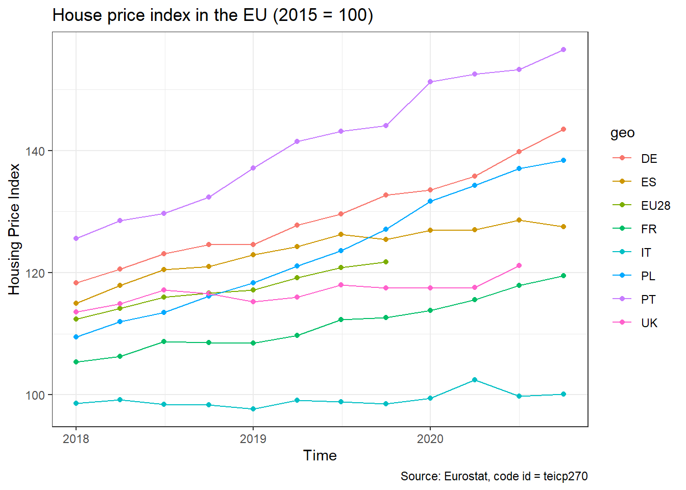
We note that our dataframe contains both the value of the index (unit = I15_NSA), as well as the percentage change (unit = PCH_Q1_NSA). We will select the I15_NSA index, a few countries and the EU-28 index, and plot the evolution of house prices over time.
hpi_data <- hpi %>%

  # choose the UK, France, Poland, Spain, Portugal, Germany, Italy, and the EU28
  filter(geo %in%  c("UK", "FR", "PL", "ES","PT", "DE","IT","EU28") ) %>%

  # choose value of the index (unit =   `I15_NSA`)
    filter(unit == "I15_NSA")

ggplot(hpi_data, aes(x=time, y=values, group=geo, colour=geo))+
  geom_point()+
  geom_line()+
  theme_bw()+
  labs(
    title= "House price index in the EU (2015 = 100)",
    x = "Time",
    y = "Housing Price Index",
    caption = "Source: Eurostat, code id = teicp270"
  )
Tourism Seasonality in the Meditteranean
The eurostat database has a dedicated tourism section.
I wanted to check monthly nights spent at hotels– the relevant code id = tour_occ_nim in the four Mediterranean countries, Portugal, Spain, Italy, and Greece since 2000.
The code below downloads the data and plots time series plots for all countries.
# create a dataframe tourism_data that contains the Eurostat data for
# code id = "tour_occ_nim", namely value of monthly nights spent at hotels
tourism_data <- get_eurostat(id="tour_occ_nim")

med_tourism <-  tourism_data %>%

  # choose Portugal, Spain, Italy, and Greece
  filter(geo %in%  c("PT", "ES", "IT", "EL" ) ) %>%

  #use label_eurostat to get verbose descriptions of codes
  label_eurostat() %>%

  # choose number of total hotel accommodations since Jan 1, 2000
  filter (c_resid == "Total",
          nace_r2 == "Hotels and similar accommodation",
          unit == "Number",
          time >= "2000-01-01") %>%

  # express values in million of nights
  mutate(values = values/1000000)

ggplot(med_tourism, aes(x=time, y=values, group=geo, colour=geo))+
  geom_point()+
  geom_line()+
  geom_smooth(se=FALSE)+
  facet_wrap(~geo)+
  theme_bw()+
  labs(title="Hotel stays in the Medditeranean, 2000-present",
       y= "Millions of nights spent in hotels",
       x = "Year",
       caption = "Source: Eurostat, code = tour_occ_nim")+
  theme(legend.position="none")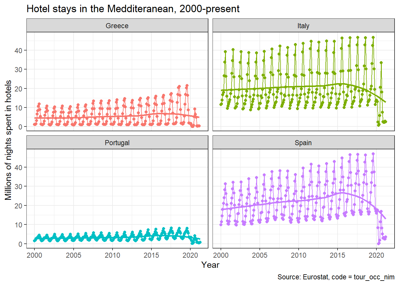
All countries exhibit the same seasonal pattern: there is a peak in July-August, and the minimum number is around December-January.
Look at the impact of Covid-19 on all countries!
#first define **ts** (time series ) objects; one for each country

portugal_tourism <- med_tourism %>%

  #select the country you are interested in, in this case Portugal
  filter (geo == "Portugal") %>%

  #sort by time in ascending order, so  earliest observation is first
  arrange(time) %>%

  #we just want to keep the values
  select(values) %>%

  #time series (ts) starts Jan 2000 and has monthlyfrequency (12 months/yr)
  ts(start=2000, frequency = 12)


spain_tourism <- med_tourism %>%
  filter (geo == "Spain") %>%
  arrange(time) %>%
  select(values) %>%
  ts(start=2000, frequency = 12)

italy_tourism <- med_tourism %>%
  filter (geo == "Italy") %>%
  arrange(time) %>%
  select(values) %>%
  ts(start=2000, frequency = 12)

greece_tourism <- med_tourism %>%
  filter (geo == "Greece") %>%
  arrange(time) %>%
  select(values) %>%
  ts(start=2000, frequency = 12)


#Season plot for Spain and Greece: the seasonal pattern is consistent since 2000
ggseasonplot(spain_tourism, year.labels=TRUE, year.labels.left=TRUE) +
  labs(
    title = "Seasonal plot: Hotel stays in Spain",
    y = "Millions of nights spent in hotels"
  )+
    theme_bw()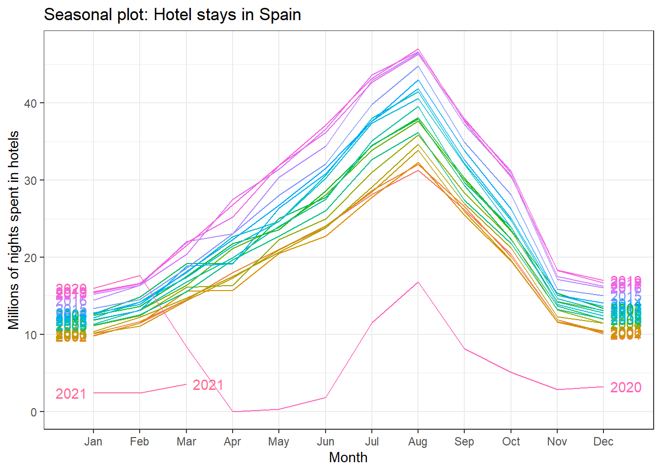
ggseasonplot(greece_tourism, year.labels=TRUE, year.labels.left=TRUE) +
  labs(
    title = "Seasonal plot: Hotel stays in Greece",
    y = "Millions of nights spent in hotels"
  )+
  theme_bw()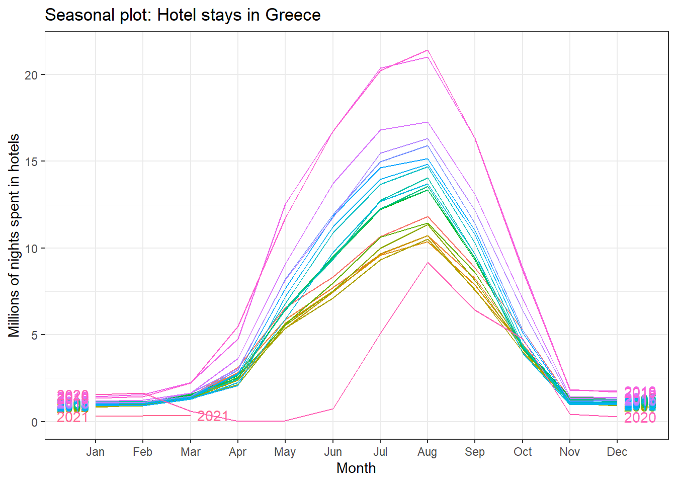
An interesting question is which country has the greatest seasonality distortion, namely, how much bigger is the summer peak from the winter bottom. For this we produce a subseries plot, one that emphasises the seasonal patterns and where the data for each season are collected together in separate mini time plots. The horizontal lines indicate the means for each month. This form of plot enables the underlying seasonal pattern to be seen clearly, and also shows the changes in seasonality over time. It is especially useful in identifying changes within particular seasons.
ggsubseriesplot(portugal_tourism)+
  labs(
    title = "Seasonal subseries plot: Hotel stays in Portugal 2000-present",
    subtitle = "Horizontal lines indicate monthly averages",
    y = "Millions of nights spent in hotels",
    caption = "Source:Eurostat"
  )+
  theme_bw()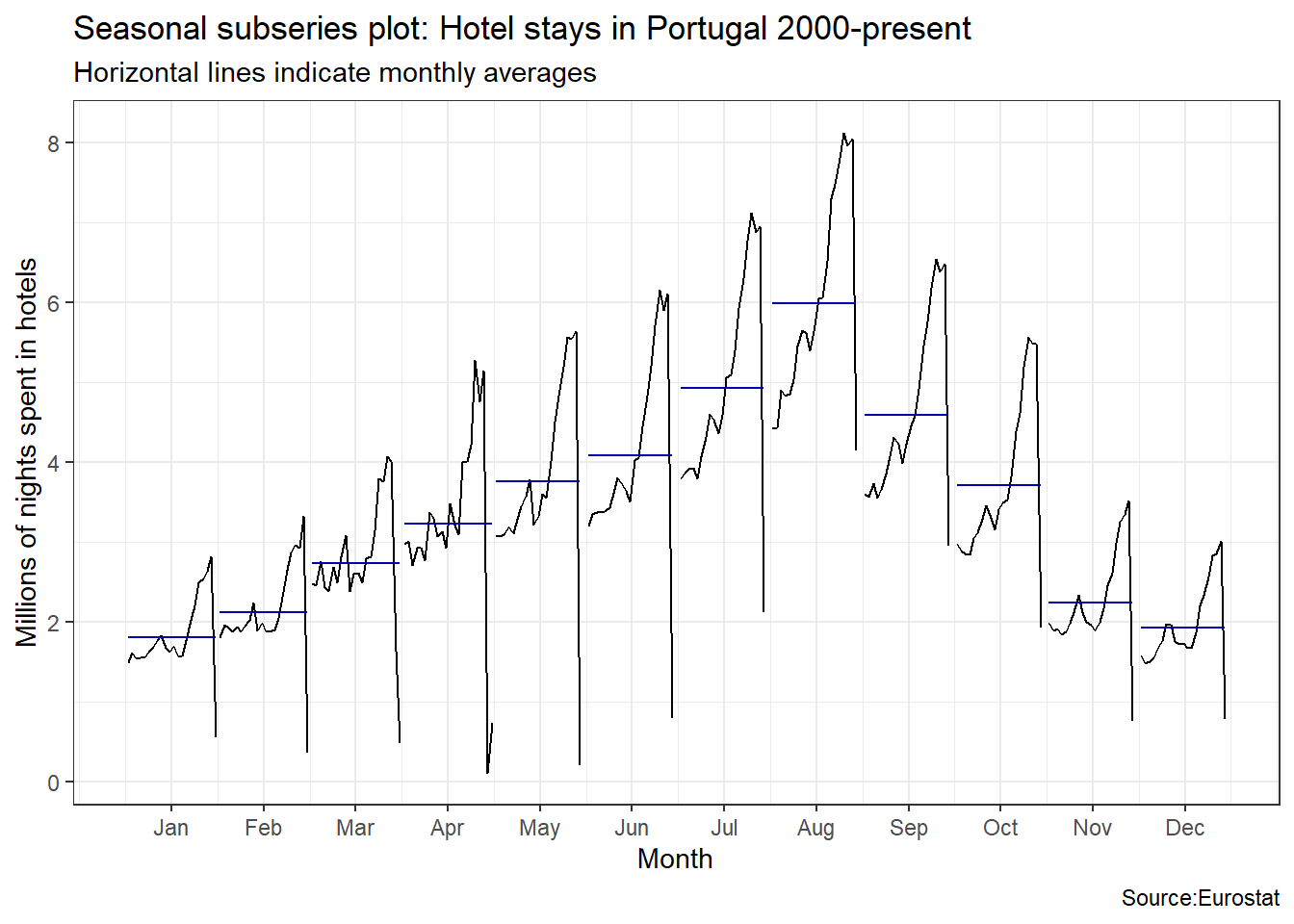
ggsubseriesplot(spain_tourism)+
  labs(
    title = "Seasonal subseries plot: Hotel stays in Spain 2000-present",
    subtitle = "Horizontal lines indicate monthly averages",
    y = "Millions of nights spent in hotels",
    caption = "Source:Eurostat"
  )+
  theme_bw()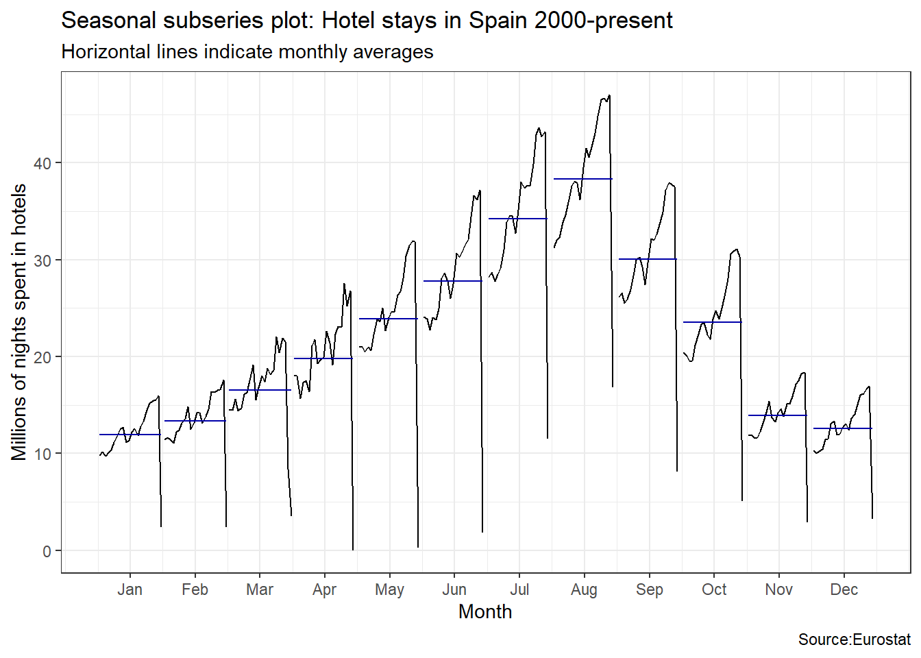
ggsubseriesplot(italy_tourism)+
  labs(
    title = "Seasonal subseries plot: Hotel stays in Italy 2000-present",
    subtitle = "Horizontal lines indicate monthly averages",
    y = "Millions of nights spent in hotels",
        caption = "Source:Eurostat"
  )+
  theme_bw()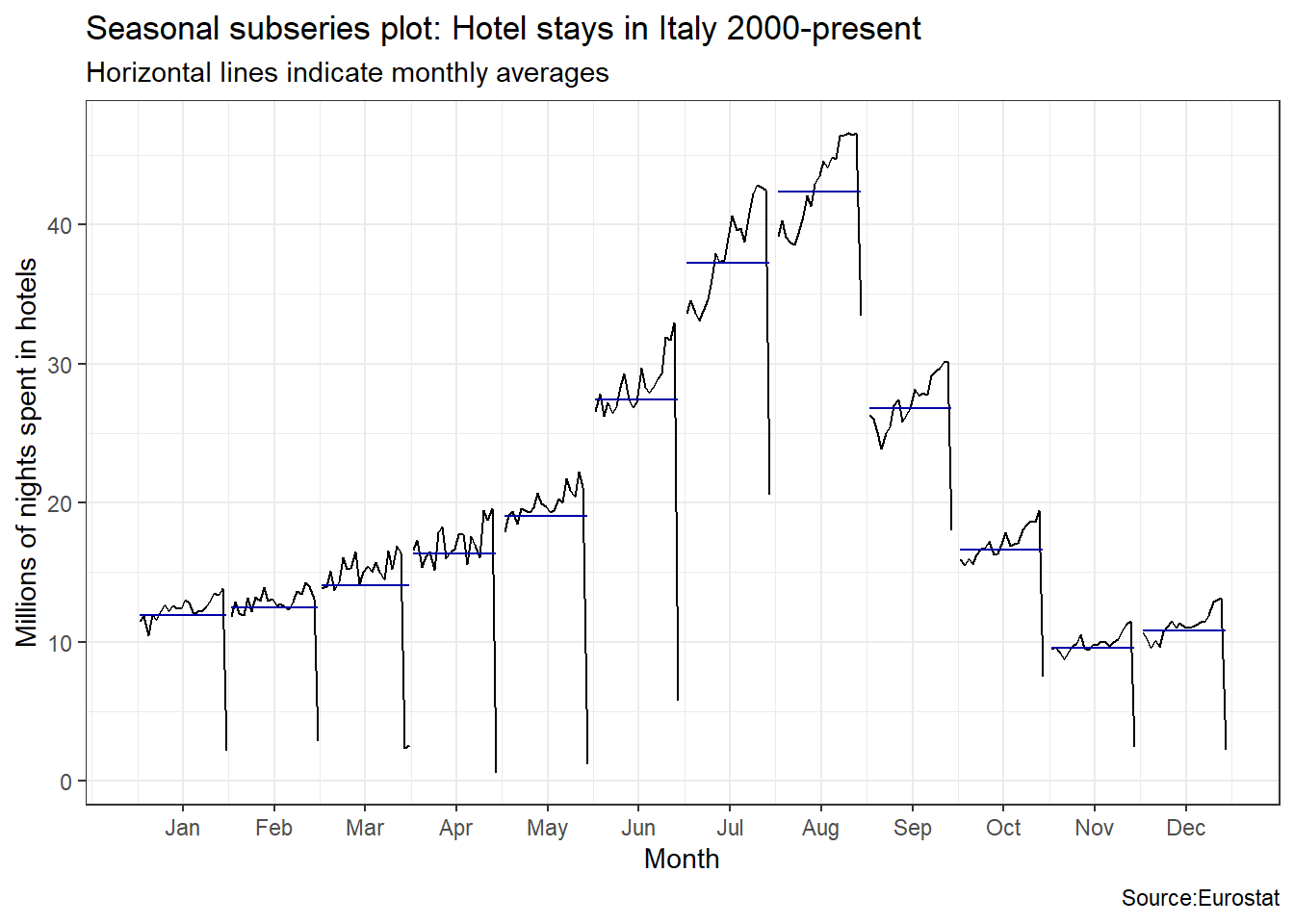
ggsubseriesplot(greece_tourism)+
  labs(
    title = "Seasonal subseries plot: Hotel stays in Greece 2000-present",
    subtitle = "Horizontal lines indicate monthly averages",
    y = "Millions of nights spent in hotels",
    caption = "Source:Eurostat"
  )+
  theme_bw()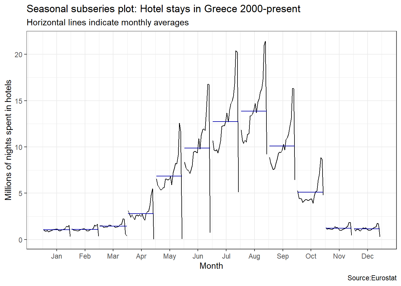
Visually, the approximate ratio of max:min averages for each of the four Mediterranean countries is as follows:
- Portugal 6:2 = 3
- Spain 39:13 = 3
- Italy 43:10 = 4.3
- Greece 13.5:1= 13.5
Disposable income of private households by NUTS 2 regions
Using the eurostat data, we can create maps of, e.g., disposable income at a regional level. NUTS or Nomenclature of Territorial Units for Statistics is a geocode standard for referencing subdivisions (regions, counties, districts, etc.) within a country.
We will work with the Disposable income of private households by NUTS 2 regions database
income_data <- get_eurostat(id="tgs00026") %>%
  select(geo,time,values) %>%
  dplyr::mutate(cat = cut_to_classes(values))


income_2016 <- income_data %>%
  filter(time == "2016-01-01")

# Download geospatial data from GISCO
geodata <- get_eurostat_geospatial(output_class = "sf",
                                   resolution = "60",
                                   nuts_level = 2,
                                   year = 2016)


map_data <- inner_join(geodata, income_2016)


ggplot(data=map_data) + geom_sf(aes(fill=cat),color="dim grey", size=.1) +
  scale_fill_brewer(palette = "Accent") +
  guides(fill = guide_legend(reverse=T, title = "euro")) +
  labs(title="Disposable household income in 2016",
       caption="(C) EuroGeographics for the administrative boundaries
                Map produced in R with a help from Eurostat-package <github.com/ropengov/eurostat/>") +
  theme_light() + theme(legend.position=c(.8,.8)) +
  coord_sf(xlim=c(-12,44), ylim=c(35,70))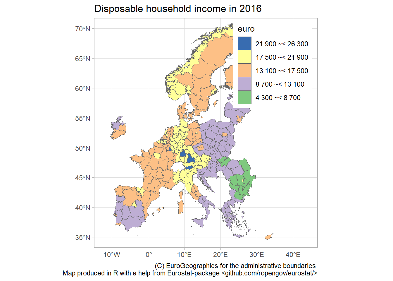
Acknowledgments
- This page is derived in part from Tutorial (vignette) for the
eurostatR package.