Using R Markdown
Reproducibility in scientific research
Reproducibility is the idea that data analyses, and more generally scientific claims, are published with their data and software code so that others may try to replicate the same work, get similar results, and build upon the works of others.
While this sounds obvious, it actually happens far less frequently than what it should.
For instance, scientists at the biotechnology company Amgen were unable to replicate the majority of published pre-clinical cancer research studies; as a matter of fact, only 6 out of 53 landmark results could be reproduced. Similarly, it has been argued that the great majority of preclinical results cannot be reproduced, leading to an annual estimate of the cost of irreproducibility on preclinical research industry to be equal to 28 Billion USD.
“You are always working with at least one collaborator: Future you.”
– Hadley Wickham
Suppose that your colleague sends you an Excel file with an analysis she has undertaken. The Excel file is likely to contain the raw data, but also graphs, results, etc. that were generated from the data. If you have ever received such an Excel analysis file, it takes a long time to navigate around it and try to understand the logic used to arrive at the results.
Data analysts who implement reproducibility in their projects can quickly and easily reproduce the original results and trace back to determine how they were derived. Literate programming, an idea from Donald Knuth, is a technique for mixing written text, where you write notes explaining what you did and why, and chunks of code that produce your graphs, analyses, etc.
This makes documentation of code easier, enables verification and replication, and allows the analyst to precisely replicate her analysis. This is extremely important when revisiting work done months later, because it’s highly likely you won’t remember how all the code/analysis works together when completing your work.
Let us change our traditional attitude to the construction of programs: Instead of imagining that our main task is to instruct a computer what to do, let us concentrate rather on explaining to humans what we want the computer to do.
– Donald E. Knuth (1984), Literate Programming
Reproducibility is also key for communicating findings with other and decision makers; it allows them to follow your logic and verify your results, assess your assumptions, and understand how your answers were formed rather than solely relying on your claimed results. In the data science framework employed in R for Data Science, reproducibility is infused throughout the entire workflow.
Your reproducibility goals should be:
- Are the results (tables and figures) reproducible from the code and data?
- Does the code actually do what you think it does?
- Is the code well documented so someone else can follow your work?
- In addition to what was done, is it clear why it was done? (e.g., how were parameter settings chosen?)
- Can the code be used for other, or newer, data?
- Can you generalise the code to do other things?
R Markdown = Markdown + R Code
R Markdown is regular Markdown with R code and output sprinkled in. You can do everything you can with regular Markdown, but you can incorporate graphs, tables, and other R output directly in your document. You can create HTML, PDF, and Word documents, PowerPoint and HTML presentations, websites, books, and even interactive dashboards with R Markdown. This whole course website is created with R Markdown (and a package named blogdown).
rmarkdown and knitr is a powerful combination of packages for literate programming, reproducible analysis, and document generation, which can:
- Combine R code and Markdown syntax
- Produce documents in PDF , Microsoft Word and various types of HTML documents
- In HTML format, it can incorporate “extras” like interactive graphics
An R Markdown file is a plain text file that uses the extension .Rmd and contains three (3) major components:
- A YAML header surrounded by
---s. This is the metadata of the document and it tells you how it is formed - what the title is, the author, date, output, and other control information.
- Chunks of R code surrounded by
``` - Text mixed with simple text formatting using the Markdown syntax
Code chunks are interspersed with text throughout the document. To complete the document, you “Knit” or “render” the document. Most of you probably knit the document by clicking the “Knit” button in the script editor panel. You can also do this programmatically from the console by running the command rmarkdown::render("example.Rmd").
When you knit the document you send your .Rmd file to knitr, a package for R that executes all the code chunks and creates a second markdown document (.md). That markdown document is then passed onto pandoc, a document rendering software program independent from R. Pandoc allows users to convert back and forth between many different document formats such as HTML, \(\LaTeX\), Microsoft Word, etc. By splitting the workflow up, you can convert your R Markdown document into a wide range of output formats.

The documentation for R Markdown is extremely comprehensive, and their tutorials and cheatsheets are excellent—rely on those.
Here are the most important things you’ll need to know about R Markdown in this class:
Key terms
Document: A Markdown file where you type stuff
Chunk: A piece of R code that is included in your document. It looks like this:
```{r chunk_name}
# Code goes here
```
There must be an empty line before and after the chunk. The final three backticks must be the only thing on the line—if you add more text, or if you forget to add the backticks, or accidentally delete the backticks, your document will not knit correctly.
Knit: When you “knit” a document, R runs each of the chunks sequentially and converts the output of each chunk into Markdown. R then runs the knitted document through pandoc to convert it to HTML or PDF or Word (or whatever output you’ve selected).
You can knit by clicking on the “Knit” button at the top of the editor window, or by pressing
⌘⇧Kon macOS orcontrol + shift + Kon Windows.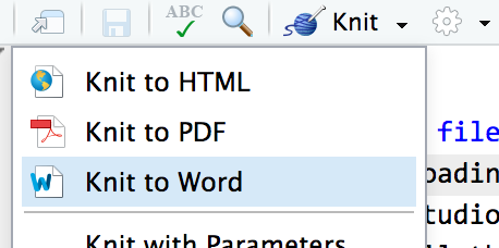
Add chunks
There are three ways to insert chunks:
Press
⌘⌥Ion macOS orcontrol + alt + Ion WindowsClick on the “Insert” button at the top of the editor window
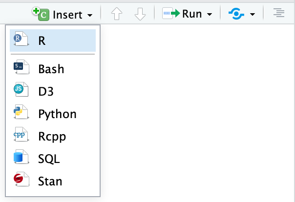
Manually type all the backticks and curly braces (don’t do this)
Chunk names
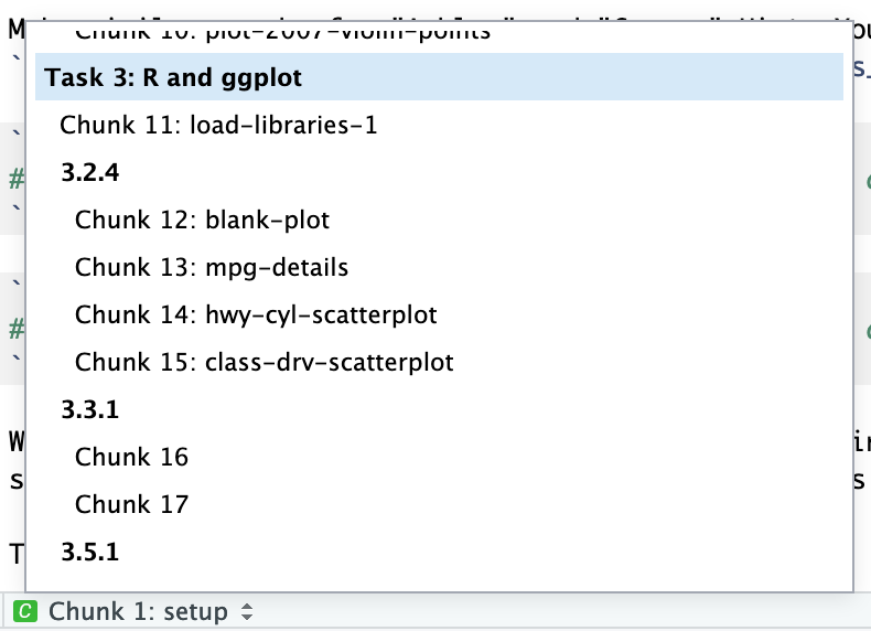
You can add names to chunks to make it easier to navigate your document. If you click on the little dropdown menu at the bottom of your editor in RStudio, you can see a table of contents that shows all the headings and chunks. If you name chunks, they’ll appear in the list. If you don’t include a name, the chunk will still show up, but you won’t know what it does.
To add a name, include it immediately after the {r in the first line of the chunk. Names cannot contain spaces, but they can contain underscores and dashes. All chunk names in your document must be unique.
A word of caution: If you use the same chunk name more than once,
knitrwill give you an error message and refuse to knit your Rmd document. So ifyou copy/paste a named chunk, make sure you give them unique names.
```{r name-of-this-chunk}
# Code goes here
```
Chunk options
There are a bunch of different options you can set for each chunk. You can see a complete list in the RMarkdown Reference Guide or at knitr’s website.
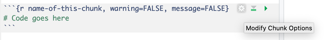
Options go inside the {r} section of the chunk:
```{r name-of-this-chunk, warning=FALSE, message=FALSE}
# Code goes here
```
The most common chunk options are these:
fig.width=5andfig.height=3(or whatever number you want): Set the dimensions for figuresecho=FALSE: The code is not shown in the final document, but the results are.include=FALSE: The chunk still runs, but the code and results are not included in the final documentmessage=FALSE: Any messages that R generates (like all the notes that appear after you load a package) are omittedwarning=FALSE: Any warnings that R generates are omittedeval = FALSE- prevents code from being evaluated. I use this in my notes for class when I want to show how to write a specific function but don’t need to actually use it.error = TRUE- causes the document to continue knitting and rendering even if the code generates a fatal error. If you’re debugging your code, you might want to use this option. However, for the final version of your work, you do not want to allow errors to pass through unnoticed.
You can also set chunk options by clicking on the little gear icon in the top right corner of any chunk:
Inline chunks
You can also include R output directly in your text, which is really helpful if you want to report numbers from your analysis. To do this, use `r r_code_here`.
It’s generally easiest to calculate numbers in a regular chunk beforehand and then use an inline chunk to display the value in your text. For instance, this document…
```{r find-avg-mpg, echo=FALSE}
avg_mpg <- mean(mtcars$mpg)
```

The average fuel efficiency for cars from 1974 was `r round(avg_mpg, 1)` miles per gallon.
… would knit into this:
The average fuel efficiency for cars from 1974 was 20.1 miles per gallon.
Caching
By default, every time you knit a document R starts anew and no previous results are saved.
If you have code chunks that run computationally intensive tasks, like running a ggpairs() correlation/scatterplot matrix in a large dataset, you might want to store these results to be more efficient and save time. If you use cache = TRUE, R will do exactly this. The output of the chunk will be saved to a specially named file on disk. Now, every time you knit the document the cached results will be used instead of running the code fresh.
Output formats
You can specify what kind of document you create when you knit in the YAML front matter.
title: "My document"
output:
html_document: default
pdf_document: default
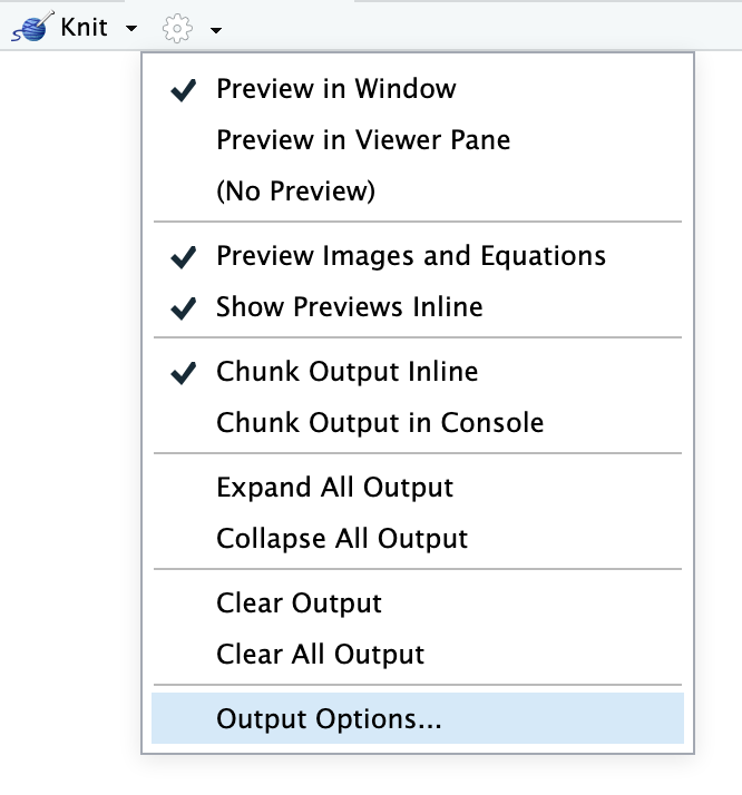
word_document: defaultYou can also click on the down arrow on the “Knit” button to choose the output and generate the appropriate YAML. If you click on the gear icon next to the “Knit” button and choose “Output options”, you change settings for each specific output type, like default figure dimensions or whether or not a table of contents is included.
The first output type listed under output: will be what is generated when you click on the “Knit” button or press the keyboard shortcut (⌘⇧K on macOS; control + shift + K on Windows). If you choose a different output with the “Knit” button menu, that output will be moved to the top of the output section.
The indentation of the YAML section matters, especially when you have settings nested under each output type. Here’s what a typical output section might look like:
---
title: "My document"
author: "My name"
date: "January 13, 2020"
output:
  html_document:
    toc: yes
    fig_caption: yes
    fig_height: 8
    fig_width: 10
  pdf_document:
    latex_engine: xelatex  # More modern PDF typesetting engine
    toc: yes
  word_document:
    toc: yes
    fig_caption: yes
    fig_height: 4
    fig_width: 5
---
Table of contents
Each output format has various options to customize the appearance of the final document. One option for HTML documents is to add a table of contents through the toc option. To add any option for an output format, just add it in a hierarchical format like this:
---
title: "My report"
author: "My Name"
date: 2020-07-26
output:
  html_document:
    toc: true
    toc_depth: 2
You can explicitly set the number of levels included in the table of contents with toc_depth (the default is 3).
Appearance and style
There are several options that control the visual appearance of HTML documents.
themespecifies the Bootstrap theme to use for the page (themes are drawn from the Bootswatch theme library). Valid themes includedefault,cerulean,journal,flatly,readable,spacelab,united,cosmo,lumen,paper,sandstone,simplex, andyeti.highlightspecifies the syntax highlighting style for code chunks. Supported styles includedefault,tango,pygments,kate,monochrome,espresso,zenburn,haddock, andtextmate.