Installing the tidyverse
Installing the tidyverse
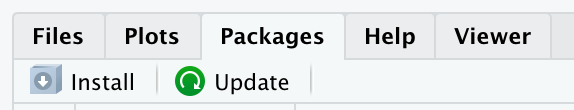
R packages are easy to install with RStudio. Select the packages panel, click on “Install,” type the name of the package you want to install, and press enter.
This can sometimes be tedious when you’re installing lots of packages, though. The tidyverse1 for instance, consists of dozens of packages that all work together. Rather than install each package individually, you can install tidyverse, a meta-package if you wish, and get them all at the same time.
Go to the packages panel in RStudio, click on “Install,” type “tidyverse”, and press enter. You’ll see a bunch of output in the RStudio console as all the tidyverse packages are installed.
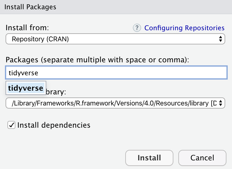
RStudio generates a line of code for you and run it: install.packages("tidyverse"). You can also just paste and run this instead of using the packages panel.
# install the major packages from the tidyverse
install.packages("tidyverse")
This will take a while as tidyverse is a collection of packages and R will have to install all dependencies.
Installing the tidyverse if you have a Mac
Unfortunately, installing the tidyverse isn’t quite always a straight-forward task with the current version of macOS 10.14, Mojave which was released on September 24, 2018.
To solve issues that may arise with missing xml2 library, please do the following:
- Open Terminal (the tab right next to Console)
- Type
xcode-select --installBe careful as you do need two (2) dashes before the install. A software update popup window should appear that will ask if you want to install command line developer tools. Click on “Install” (you don’t need to click on “Get Xcode”)
- Go to https://brew.sh and copy the long command under “Install Homebrew” (starts with
/usr/bin/ruby -e "$(curl -fsSL.), paste it into Terminal, and press enter.
/usr/bin/ruby -e "$(curl -fsSL https://raw.githubusercontent.com/Homebrew/install/master/install)"This installs Homebrew, which is special software that lets you install Unix-y programs from the terminal.
- Type the following command line in Terminal to install
libxml2
brew install libxml2 - Then, within RStudio, type
install.packages("xml2") - Finally, you can now proceed with the installation of the
tidyverse
install.packages("tidyverse")Installing further packages
Once the tidyverse collection of packages installs and you get back to the R prompt >, you can install a series of packages that will be useful later in the course. You can copy/paste the code below; please note that this will take quite a while, so grab a coffee.
# install these packages as well
list_of_packages <- c(
  "moderndive",   # https://www.moderndive.com/
  "DT",           # Allows us to handle Data Tables and manipulate data faster
  "unvotes",      # How countries have voted in UN resolutions
  "gridExtra",    # Miscellaneous Functions for "Grid" Graphics
  "GGally",       # Allows us to create a correlations/scatterplots matrix
  "tidyquant",    # Download and manipulate financial data
  "wbstats",      # Download World Bank Data
  "eurostat",     # Download data from Eurostat
  "fpp2",         # Time Series and Forecasting fucntions, with data too
  "car",          # Applied Regression- allows to calculate VIF, Variance Inflation Factor
  "gapminder",    # Data on life expectancy, GDP/capita, and population by country and year
  "nycflights13", # Data on all domestic flights through NYCs 3 airports (JFK, EWR, LGA) in 2013
  "fivethirtyeight", #Data used in articles that appeared in the fivethirtyeight.com website
  "corrr",        # correlation in R
  "plotly",       # interactive visualizations
  "sf",           # tidy geo-computing
  "cowplot",      # ggplot multiple figures addon
  "coefplot",     # plot coefficients from fitted models
  "interplot",    # plot effects of variables in interaction terms
  "scales",       # scale functions for visualisations
  "ggridges",     # ridgeline plots in ggplot2
  "skimr",        # nice dataframe summaries
  "leaflet",      # interactive maps
  "ggrepel",      # geoms for ggplot2 to repel overlapping text labels
  "viridis",      # Colour Maps
  "rvest",        # scrape webpages
  "usethis",      # automation of package and project setup
  "remotes",      # installing packages from Github
  "tidytext",     # text mining
  "here",         # finding your files
  "mosaic"        # summary stats, using mosaic::favstats()
)

install.packages(list_of_packages, dependencies=TRUE, repos = "https://cran.rstudio.com/")
Install from Github
Most of the time the packages that you’ll want to install have been made available on CRAN, the Comprehensive R Archive Network, so you use the install.packages("package_name") function. Sometimes people write packages that are not submitted to CRAN, and sometimes you might want to try out a package that is currently under development. In these situations, people who write packages will often make them available on GitHub. We can install packages directly from Github, using the devtools package.
The first thing you need to do is install remotes, which is easy because that package is available on CRAN and hopefully you installed it with all packages listed earlier. If not,
install.packages("remotes")Once you install remotes, you must explicitly say to R you will be using it by typing library(devtools). Then, you can use the install_github command to install a package directly from a GitHub repository. For example, there’s an R data package featuring every Lego set from 1970 to 2015 put together by Sean Kross.
remotes::install_github("seankross/lego") #install the lego package directly from Github R fetches and installs the package from Github, and we now have the new lego package to play with. To verify that everything worked properly, let’s load the lego package and look at its legosets dataframe:
library(lego)     #load the lego package into the computer's memory

legosets          #view the legosets dataframe
## # A tibble: 6,172 x 14
## Item_Number Name Year Theme Subtheme Pieces Minifigures Image_URL GBP_MSRP
## <chr> <chr> <int> <chr> <chr> <int> <int> <chr> <dbl>
## 1 10246 Dete~ 2015 Adva~ "Modula~ 2262 6 http://i~ 133.
## 2 10247 Ferr~ 2015 Adva~ "Fairgr~ 2464 10 http://i~ 150.
## 3 10248 Ferr~ 2015 Adva~ "Vehicl~ 1158 NA http://i~ 70.0
## 4 10249 Toy ~ 2015 Adva~ "Winter~ 898 NA http://i~ 60.0
## 5 10581 Ducks 2015 Duplo "Forest~ 13 1 http://i~ 9.99
## 6 10582 Anim~ 2015 Duplo "Forest~ 39 2 http://i~ 17.0
## 7 10583 Fish~ 2015 Duplo "Forest~ 32 2 http://i~ 20.0
## 8 10584 Fore~ 2015 Duplo "Forest~ 105 3 http://i~ 50.0
## 9 10585 Mom ~ 2015 Duplo "" 13 2 http://i~ 8.99
## 10 10586 Ice ~ 2015 Duplo "" 11 2 http://i~ 13.0
## # ... with 6,162 more rows, and 5 more variables: USD_MSRP <dbl>,
## # CAD_MSRP <dbl>, EUR_MSRP <dbl>, Packaging <chr>, Availability <chr>glimpse(legosets) #examine the structure of the dataframe- variables, observations, type of variables, etc.## Rows: 6,172
## Columns: 14
## $ Item_Number <chr> "10246", "10247", "10248", "10249", "10581", "10582", ...
## $ Name <chr> "Detective's Office", "Ferris Wheel", "Ferrari F40", "...
## $ Year <int> 2015, 2015, 2015, 2015, 2015, 2015, 2015, 2015, 2015, ...
## $ Theme <chr> "Advanced Models", "Advanced Models", "Advanced Models...
## $ Subtheme <chr> "Modular Buildings", "Fairground", "Vehicles", "Winter...
## $ Pieces <int> 2262, 2464, 1158, 898, 13, 39, 32, 105, 13, 11, 52, 13...
## $ Minifigures <int> 6, 10, NA, NA, 1, 2, 2, 3, 2, 2, 3, 1, NA, NA, NA, NA,...
## $ Image_URL <chr> "http://images.brickset.com/sets/images/10246-1.jpg", ...
## $ GBP_MSRP <dbl> 132.99, 149.99, 69.99, 59.99, 9.99, 16.99, 19.99, 49.9...
## $ USD_MSRP <dbl> 159.99, 199.99, 99.99, 79.99, 9.99, 19.99, 24.99, 59.9...
## $ CAD_MSRP <dbl> 199.99, 229.99, 119.99, NA, 12.99, 24.99, 29.99, 69.99...
## $ EUR_MSRP <dbl> 149.99, 179.99, 89.99, 69.99, 9.99, 19.99, 24.99, 59.9...
## $ Packaging <chr> "Box", "Box", "Box", "Box", "Box", "Box", "Box", "Box"...
## $ Availability <chr> "Retail - limited", "Retail - limited", "LEGO exclusiv...The dataframe has 14 variables (or columns) and 6,172 observations (rows). Besides the item number, year, theme/subtheme and the number of pieces and minifigures contained in each Lego box, we also have the recommended retail prices in GBP, USD, CAD, and EUR. While we are at it, let us have a quick look at how Lego prices (in GBP) have evolved over the years.
avg_price_per_year <- legosets %>% # create avg_price_year" by taking legosets, and then
  filter(!is.na(GBP_MSRP)) %>%    # filter out entries with no GBP prices, GBP_MSRP, and then
  group_by(Year) %>%              # group prices by year
  summarise(Price = mean(GBP_MSRP)) # create variable "Price" = yearly average of GBP_MSRP

ggplot(avg_price_per_year,
       mapping = aes(x = Year, y = Price)) +  # time series plot: x=Year, y=Price
  geom_point(size = 0.5) +                    # simple scatterplot Y vs. X
  geom_line(size = 0.5) +                     # add the black line between points
  geom_smooth(se = FALSE) +                   # fit trend line,no error band around it "se = FALSE"
  labs(x = "Year",
       y = "Price (GBP)",
       title = "Average price of LEGO sets",
       subtitle = "Amounts are reported in current GBP",
       caption = "Source: LEGO") +
  theme_bw()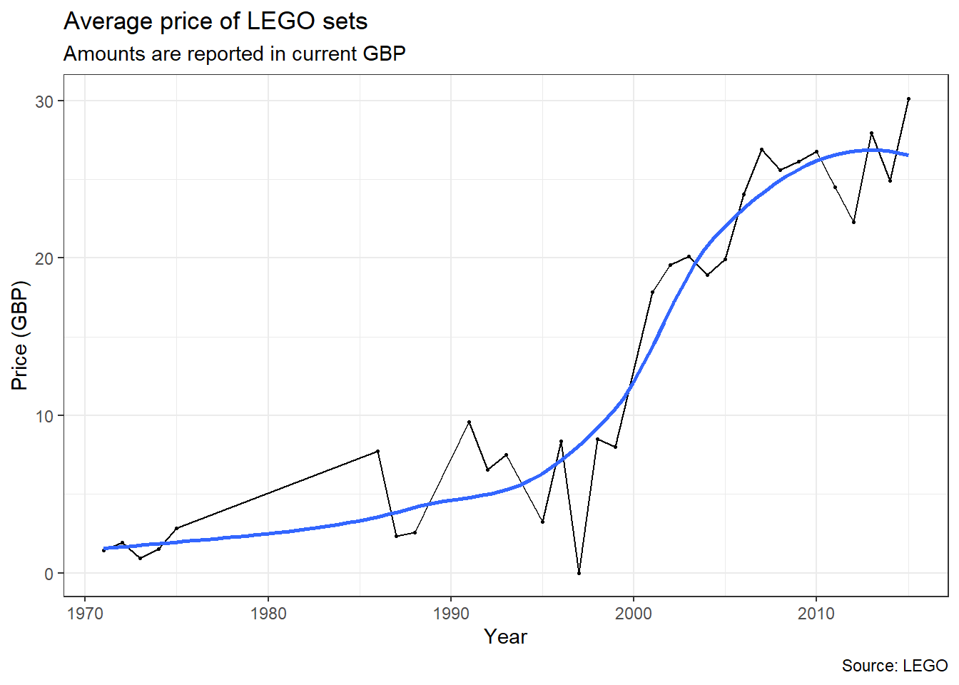
There is a clear upward trend in average GBP prices.
And since we are talking about LEGOs, here is a fun application of creating LEGO mosaics from photos using R & the tidyverse
Updating packages
Every now and then the authors of packages release updated versions. The updated versions often add new functionality, fix bugs, and so on. It’s a good idea to update your packages periodically.
There’s an update.packages function, but it’s probably easier to stick with the RStudio tool. In the packages tab, click on the Update Packages button. This will bring up a window that looks like the one shown below:
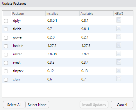
In this window, each row refers to a package that needs to be updated. You can select which updates to install by checking the boxes on the left. If you feel lazy, click the Select All button, and then Install Updates. This might take a while to complete depending on how fast your internet connection is.
Updating R
About twice a year, a new version of R is released, and the features of all packages get changed to be compatible with the new version of R. The side effect of packages being compatible with the newest R version is that then you update to the newest version of R, you lose all the packages that you have downloaded and installed. Unfortunately, you need to install the new versions of packages, even though they will typically behave just like the old ones.
Install tinytex
When you knit to PDF, R uses a special scientific typesetting program named LaTeX (pronounced “lay-tek” or “lah-tex”; for goofy nerdy reasons, the x is technically the “ch” sound in “Bach”, but most people just say it as “k”—saying “layteks” is frowned on for whatever reason).
LaTeX makes pretty documents, but it’s a huge program—the macOS version, for instance, is nearly 4 GB! To make life easier, there’s an R package named tinytex that installs a minimal LaTeX program and that automatically deals with differences between macOS and Windows.
Here’s how to install tinytex so you can knit to pretty PDFs:
- Use the Packages in panel in RStudio to install tinytex like you did above with tidyverse. Alternatively, run
install.packages("tinytex")in the console. - Run
tinytex::install_tinytex()in the console. - Wait for a bit while R downloads and installs everything you need.
- The end! You should now be able to knit to PDF.
A universe of packages centered around tidy data, including
ggplot2↩︎