Linear Model Fitting
- Fit a model using
lm(Y ~ X1 + X2 +..., data = dataframe) - Look at model output
- Write down the equation for model1
- Plot scatterplot and residuals
- Add more explanatory variables
- Check collinearity
- Summary model comparison table using
huxtable::huxreg() - Fitting multiple regression models in one go
- Simpson’s paradox
We will be using the Palmer penguins data to understand body mass.
Fit a model using lm(Y ~ X1 + X2 +..., data = dataframe)
The function to fit a linear regression model in R is lm(Y ~ X1 + X2 +..., data = mydataframe). lm, as many other functions in R, uses the formula interface The tilde (~) can be translated as is a function of. We are saying that \(Y\) is a function of \(X1\), \(X2\), etc., and the data for our analysis comes from mydataframe.
Back to our penguins, we want to see whether body mass is a function of flipper length. We create an object called model1 that holds the results of this linear regression model.
model1 <- lm(body_mass_g ~ flipper_length_mm, data = penguins)Look at model output
We will be using the broom package to make modelling easier to work with. There are 3 main functions in broom:
tidy()- This is where you get most of the output you want, including coefficients and p-valuesglance()- additional measures on your model, including R-squared, log likelihood, and AIC/BICaugment()- make predictions with your model using new data
For now, we will use broom::tidy() and broom::glance() to get model results.
model1 %>% broom::tidy()| term | estimate | std.error | statistic | p.value |
|---|---|---|---|---|
| (Intercept) | -5.78e+03 | 306 | -18.9 | 5.59e-55 |
| flipper_length_mm | 49.7 | 1.52 | 32.7 | 4.37e-107 |
model1 %>% broom::glance()| r.squared | adj.r.squared | sigma | statistic | p.value | df | logLik | AIC | BIC | deviance | df.residual | nobs |
|---|---|---|---|---|---|---|---|---|---|---|---|
| 0.759 | 0.758 | 394 | 1.07e+03 | 4.37e-107 | 1 | -2.53e+03 | 5.06e+03 | 5.07e+03 | 5.29e+07 | 340 | 342 |
Write down the equation for model1
\[ \text{body_mass_g} = \alpha + \beta_{1}(\text{flipper_length_mm}) + \epsilon \] \[ \text{body_mass_g} = -5780.83 + 49.69(\text{flipper_length_mm}) + \epsilon \]
Plot scatterplot and residuals
Add more explanatory variables
model2 <- lm(body_mass_g ~ flipper_length_mm + species , data = penguins)

model3 <- lm(body_mass_g ~ flipper_length_mm + species + sex , data = penguins)

model4 <- lm(body_mass_g ~ flipper_length_mm + species + sex + bill_length_mm, data = penguins)

model5 <- lm(body_mass_g ~ flipper_length_mm + species + sex + bill_length_mm + bill_depth_mm , data = penguins)

# Fit a model with all explanatory variables (~ .)
model6 <- lm(body_mass_g ~ . , data = penguins)
Check collinearity
With so many explanatory variables, we need to worry about colinearity, i.e., whether the explanatory variables (all of the \(X\)’s) are highly correlated among themselves.
#model2 <- lm(body_mass_g ~ flipper_length_mm + species , data = penguins)
car::vif(model2)
## GVIF Df GVIF^(1/(2*Df))
## flipper_length_mm 4.51 1 2.12
## species 4.51 2 1.46# model3 <- lm(body_mass_g ~ flipper_length_mm + species + sex , data = penguins)
car::vif(model3)## GVIF Df GVIF^(1/(2*Df))
## flipper_length_mm 6.05 1 2.46
## species 5.65 2 1.54
## sex 1.36 1 1.17# model4 <- lm(body_mass_g ~ flipper_length_mm + species + sex + bill_length_mm, data = penguins)
car::vif(model4)## GVIF Df GVIF^(1/(2*Df))
## flipper_length_mm 6.44 1 2.54
## species 18.16 2 2.06
## sex 1.81 1 1.35
## bill_length_mm 5.95 1 2.44# model5 <- lm(body_mass_g ~ flipper_length_mm + species + sex + bill_length_mm + bill_depth_mm , data = penguins)
car::vif(model5)## GVIF Df GVIF^(1/(2*Df))
## flipper_length_mm 6.69 1 2.59
## species 41.07 2 2.53
## sex 2.31 1 1.52
## bill_length_mm 6.07 1 2.46
## bill_depth_mm 6.08 1 2.47# model6 <- lm(body_mass_g ~ . , data = penguins)
car::vif(model6)## GVIF Df GVIF^(1/(2*Df))
## species 71.20 2 2.90
## island 3.76 2 1.39
## bill_length_mm 6.12 1 2.47
## bill_depth_mm 6.27 1 2.50
## flipper_length_mm 7.78 1 2.79
## sex 2.34 1 1.53
## year 1.17 1 1.08model7 <- lm(body_mass_g ~ flipper_length_mm + sex + bill_depth_mm , data = penguins)
car::vif(model7)## flipper_length_mm sex bill_depth_mm
## 2.44 1.89 2.65Summary model comparison table using huxtable::huxreg()
Which of the six models we have fit seems to be the best one? Let us compare them on one table.
huxreg(model1, model2, model3, model4, model5, model6, model7,
                 statistics = c('#observations' = 'nobs',
                                'R squared' = 'r.squared',
                                'Adj. R Squared' = 'adj.r.squared',
                                'Residual SE' = 'sigma'),
                 bold_signif = 0.05
) %>%
set_caption('Comparison of models')| (1) | (2) | (3) | (4) | (5) | (6) | (7) | |
|---|---|---|---|---|---|---|---|
| (Intercept) | -5780.831 *** | -4031.477 *** | -365.817 | -759.064 | -1460.995 * | 84087.945 * | -2246.829 *** |
| (305.815) | (584.151) | (532.050) | (541.377) | (571.308) | (41912.019) | (625.286) | |
| flipper_length_mm | 49.686 *** | 40.705 *** | 20.025 *** | 17.847 *** | 15.950 *** | 18.504 *** | 38.190 *** |
| (1.518) | (3.071) | (2.846) | (2.902) | (2.910) | (3.128) | (2.084) | |
| speciesChinstrap | -206.510 *** | -87.634 | -291.711 *** | -251.477 ** | -282.539 ** | ||
| (57.731) | (46.347) | (81.502) | (81.079) | (88.790) | |||
| speciesGentoo | 266.810 ** | 836.260 *** | 707.028 *** | 1014.627 *** | 890.958 *** | ||
| (95.264) | (85.185) | (94.359) | (129.561) | (144.563) | |||
| sexmale | 530.381 *** | 465.395 *** | 389.892 *** | 378.977 *** | 538.080 *** | ||
| (37.810) | (43.081) | (47.848) | (48.074) | (51.310) | |||
| bill_length_mm | 21.633 ** | 18.204 * | 18.964 ** | ||||
| (7.148) | (7.106) | (7.112) | |||||
| bill_depth_mm | 67.218 *** | 60.798 ** | -86.947 *** | ||||
| (19.742) | (20.002) | (15.456) | |||||
| islandDream | -21.180 | ||||||
| (58.390) | |||||||
| islandTorgersen | -58.777 | ||||||
| (60.852) | |||||||
| year | -42.785 * | ||||||
| (20.949) | |||||||
| #observations | 342 | 342 | 333 | 333 | 333 | 333 | 333 |
| R squared | 0.759 | 0.783 | 0.867 | 0.871 | 0.875 | 0.877 | 0.823 |
| Adj. R Squared | 0.758 | 0.781 | 0.865 | 0.869 | 0.873 | 0.873 | 0.821 |
| Residual SE | 394.278 | 375.535 | 295.565 | 291.955 | 287.338 | 286.524 | 340.427 |
| *** p < 0.001; ** p < 0.01; * p < 0.05. | |||||||
The best model seems to be model 7, so we will use broom::tidy() and broom::glance() to get model results.
model7 %>% broom::tidy()| term | estimate | std.error | statistic | p.value |
|---|---|---|---|---|
| (Intercept) | -2.25e+03 | 625 | -3.59 | 0.000376 |
| flipper_length_mm | 38.2 | 2.08 | 18.3 | 3.47e-52 |
| sexmale | 538 | 51.3 | 10.5 | 2.17e-22 |
| bill_depth_mm | -86.9 | 15.5 | -5.63 | 3.96e-08 |
model7 %>% broom::glance()| r.squared | adj.r.squared | sigma | statistic | p.value | df | logLik | AIC | BIC | deviance | df.residual | nobs |
|---|---|---|---|---|---|---|---|---|---|---|---|
| 0.823 | 0.821 | 340 | 509 | 2.9e-123 | 3 | -2.41e+03 | 4.83e+03 | 4.85e+03 | 3.81e+07 | 329 | 333 |
Let us write down its equation
\[ \begin{aligned} \text{body_mass_g} &= \alpha + \beta_{1}(\text{flipper_length_mm}) + \beta_{2}(\text{sex}_{\text{male}})\ + \beta_{3}(\text{bill_depth_mm}) + \epsilon \end{aligned} \]\[ \begin{aligned} \text{body_mass_g} &= -2246.83 + 38.19(\text{flipper_length_mm}) + 538.08(\text{sex}_{\text{male}})\ - 86.95(\text{bill_depth_mm}) + \epsilon \end{aligned} \]
Fitting multiple regression models in one go
Let us recall the relationship between body mass and bill depth and have a look at the scatterplot.
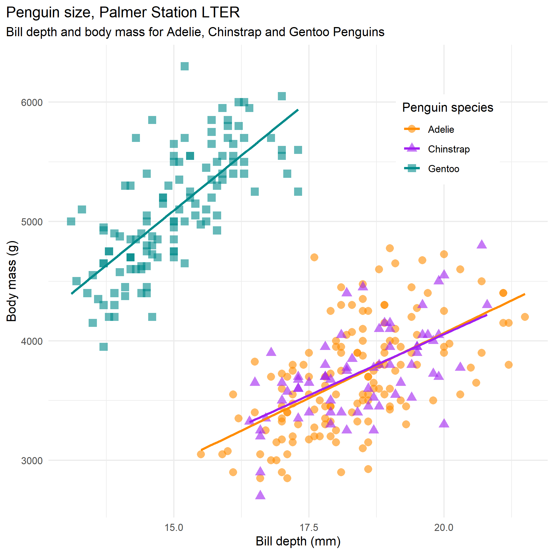
We could run three separate regression, but we can estimate three regression models with a few lines of code.
penguins %>%
  na.omit() %>%
  group_by(species) %>%
  summarise(
    broom::tidy(lm( body_mass_g ~ bill_depth_mm))
  )
## # A tibble: 6 x 6
## # Groups: species [3]
## species term estimate std.error statistic p.value
## <fct> <chr> <dbl> <dbl> <dbl> <dbl>
## 1 Adelie (Intercept) -297. 469. -0.634 5.27e- 1
## 2 Adelie bill_depth_mm 218. 25.5 8.55 1.67e-14
## 3 Chinstrap (Intercept) -36.2 613. -0.0591 9.53e- 1
## 4 Chinstrap bill_depth_mm 205. 33.2 6.16 4.79e- 8
## 5 Gentoo (Intercept) -422. 488. -0.864 3.89e- 1
## 6 Gentoo bill_depth_mm 368. 32.5 11.3 1.64e-20What we see is BLAH…
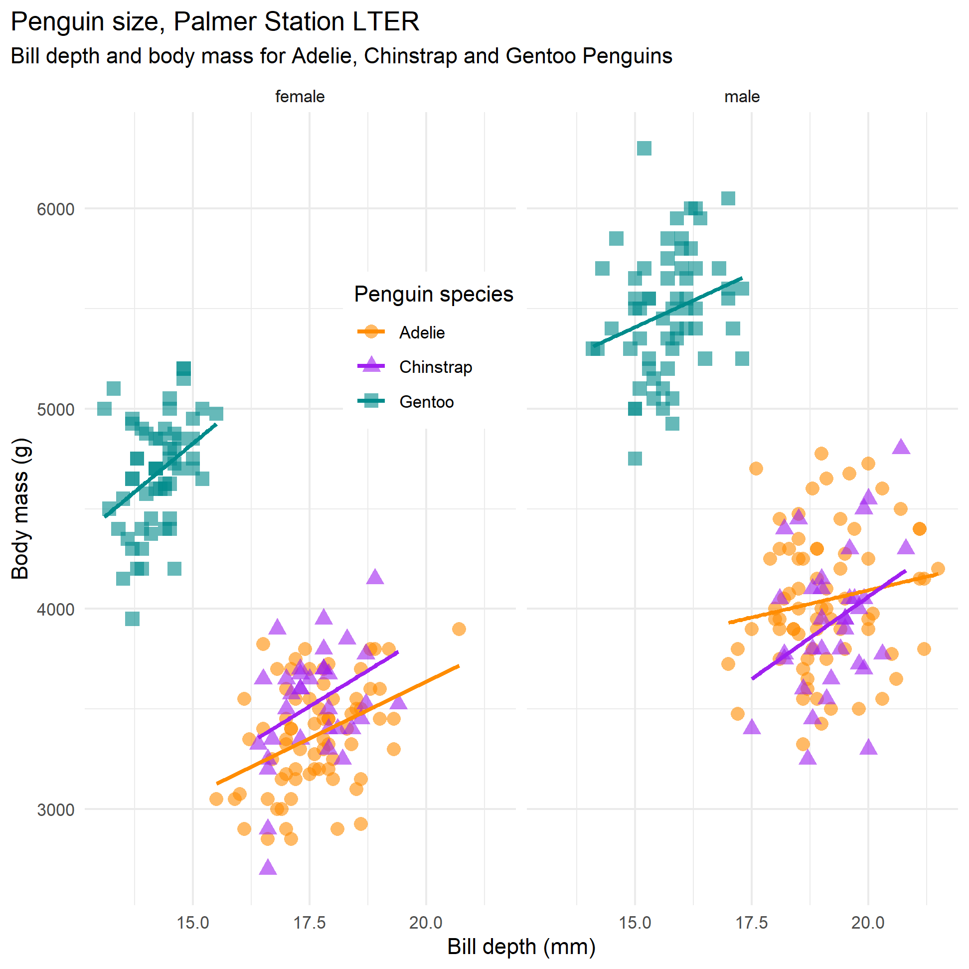
What if we add sex? First, let us facet_wrap() our scatter plot to see what it looks like
penguins %>%
  na.omit() %>%
  group_by(species) %>%
  summarise(
    broom::tidy(lm( body_mass_g ~ bill_depth_mm + sex))
  )
## # A tibble: 9 x 6
## # Groups: species [3]
## species term estimate std.error statistic p.value
## <fct> <chr> <dbl> <dbl> <dbl> <dbl>
## 1 Adelie (Intercept) 1931. 452. 4.28 3.47e- 5
## 2 Adelie bill_depth_mm 81.6 25.6 3.19 1.74e- 3
## 3 Adelie sexmale 556. 62.1 8.96 1.63e-15
## 4 Chinstrap (Intercept) 830. 861. 0.964 3.39e- 1
## 5 Chinstrap bill_depth_mm 153. 48.9 3.14 2.55e- 3
## 6 Chinstrap sexmale 156. 110. 1.42 1.60e- 1
## 7 Gentoo (Intercept) 2741. 579. 4.73 6.37e- 6
## 8 Gentoo bill_depth_mm 136. 40.6 3.35 1.08e- 3
## 9 Gentoo sexmale 604. 79.8 7.57 9.94e-12Simpson’s paradox
Recall from our EDA, we saw no relationship between bill length and depth.
bill_no_species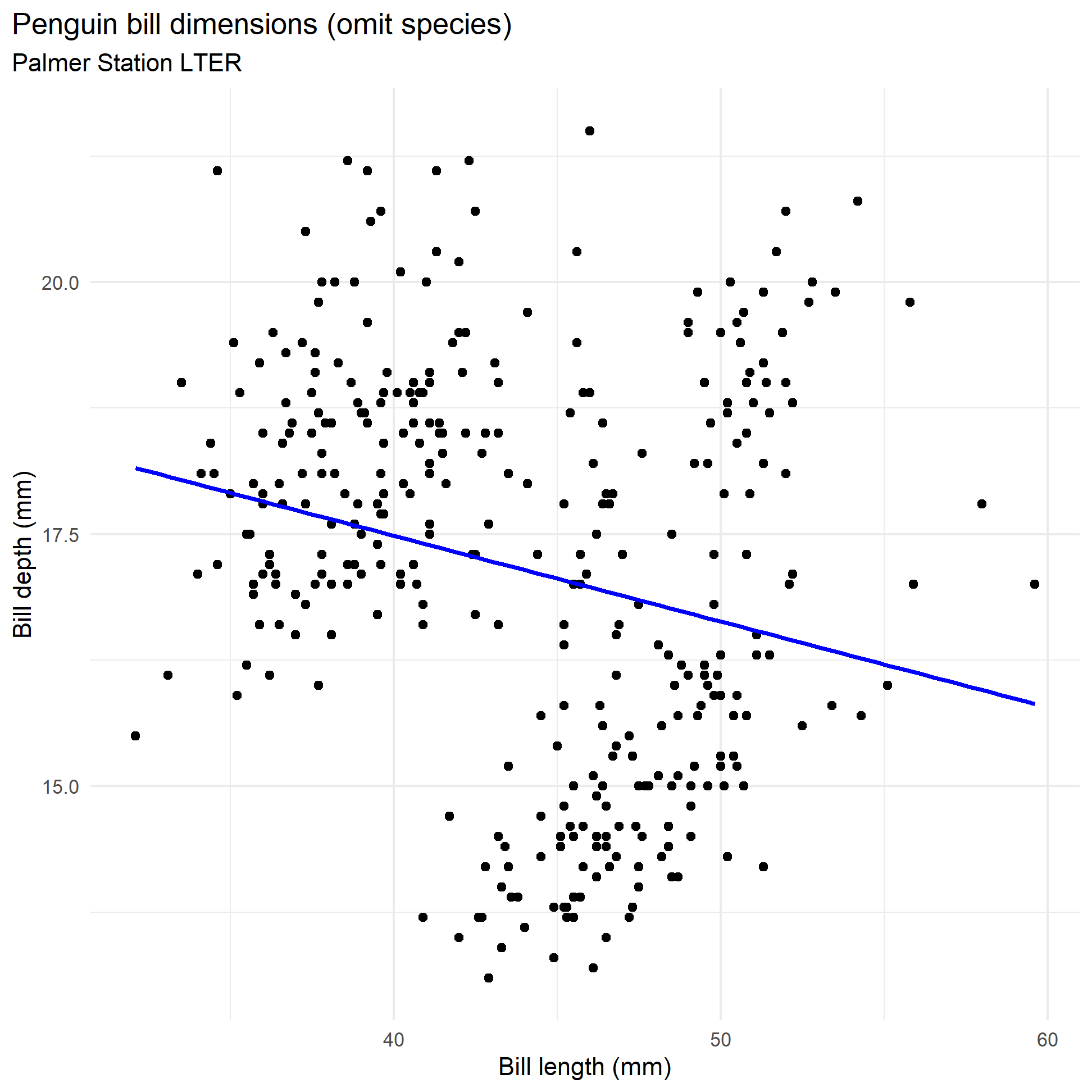
If we fit a simple regression model, we get the following
simpsons_model <- lm( bill_depth_mm ~ bill_length_mm,
                      data = penguins %>% na.omit())

simpsons_model %>% broom::tidy()| term | estimate | std.error | statistic | p.value |
|---|---|---|---|---|
| (Intercept) | 20.8 | 0.854 | 24.3 | 1.03e-75 |
| bill_length_mm | -0.0823 | 0.0193 | -4.27 | 2.53e-05 |
simpsons_model %>% broom::glance()| r.squared | adj.r.squared | sigma | statistic | p.value | df | logLik | AIC | BIC | deviance | df.residual | nobs |
|---|---|---|---|---|---|---|---|---|---|---|---|
| 0.0523 | 0.0494 | 1.92 | 18.3 | 2.53e-05 | 1 | -689 | 1.38e+03 | 1.39e+03 | 1.22e+03 | 331 | 333 |
However, when we plotted the same scatterplot colouring points by species, we got a completely different story.
bill_len_dep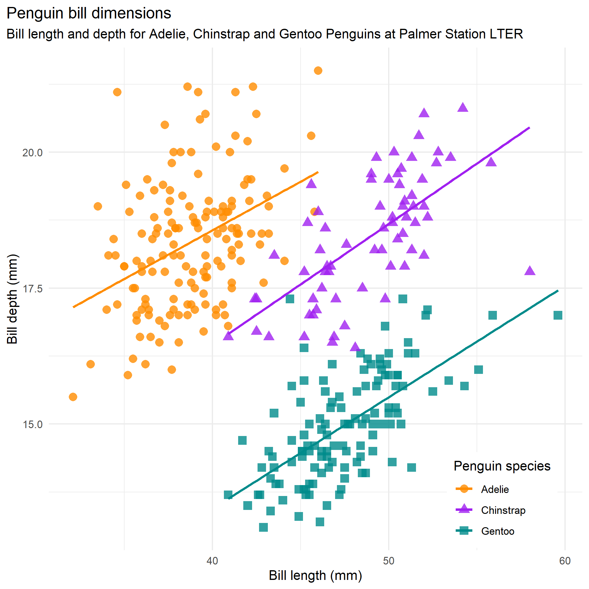
We can again fit three individual models in one go
penguins %>%
  na.omit() %>%
  group_by(species) %>%
  summarise(
    broom::tidy(lm( bill_depth_mm ~ bill_length_mm )),
    broom::glance(lm( bill_depth_mm ~ bill_length_mm ))
  )
## # A tibble: 6 x 16
## # Groups: species [3]
## species term estimate std.error statistic p.value r.squared adj.r.squared
## <fct> <chr> <dbl> <dbl> <dbl> <dbl> <dbl> <dbl>
## 1 Adelie (Int~ 11.5 1.37 25.2 1.51e- 6 0.149 0.143
## 2 Adelie bill~ 0.177 0.0352 25.2 1.51e- 6 0.149 0.143
## 3 Chinst~ (Int~ 7.57 1.55 49.2 1.53e- 9 0.427 0.418
## 4 Chinst~ bill~ 0.222 0.0317 49.2 1.53e- 9 0.427 0.418
## 5 Gentoo (Int~ 5.12 1.06 87.5 7.34e-16 0.428 0.423
## 6 Gentoo bill~ 0.208 0.0222 87.5 7.34e-16 0.428 0.423
## # ... with 8 more variables: sigma <dbl>, df <dbl>, logLik <dbl>, AIC <dbl>,
## # BIC <dbl>, deviance <dbl>, df.residual <int>, nobs <int>Alternatively, we can run a multiple regression model and the adjusted R2 = 76.5%
simpsons_model2 <- lm( bill_depth_mm ~ bill_length_mm + species,
                      data = penguins %>% na.omit())

simpsons_model2 %>% broom::tidy()| term | estimate | std.error | statistic | p.value |
|---|---|---|---|---|
| (Intercept) | 10.6 | 0.691 | 15.3 | 2.98e-40 |
| bill_length_mm | 0.2 | 0.0177 | 11.3 | 2.26e-25 |
| speciesChinstrap | -1.93 | 0.226 | -8.56 | 4.26e-16 |
| speciesGentoo | -5.1 | 0.194 | -26.3 | 1.04e-82 |
simpsons_model2 %>% broom::glance()| r.squared | adj.r.squared | sigma | statistic | p.value | df | logLik | AIC | BIC | deviance | df.residual | nobs |
|---|---|---|---|---|---|---|---|---|---|---|---|
| 0.767 | 0.765 | 0.954 | 362 | 8.88e-104 | 3 | -455 | 920 | 939 | 300 | 329 | 333 |