Model diagnostics

Linear Regression Assumptions: L-I-N-E

• L: Linear relationship between (Y) and the explanatory variable (X)
• I: Independence of errors—there’s no connection between how far any two points lie from the regression line
• N: Normal distribution of Y at each level of X
• E: equality of variance of the errors – variability remains the same for all levels of X.

In other words, the residuals (errors) should satisfy the following:

• L: The mean value for Y at each level of X lies on regression line.
• I: There is no clear pattern in the errors
• N: At each level of X, the values for Y are normally distributed.
• E: The variability in the Y’s for each level of X is the same

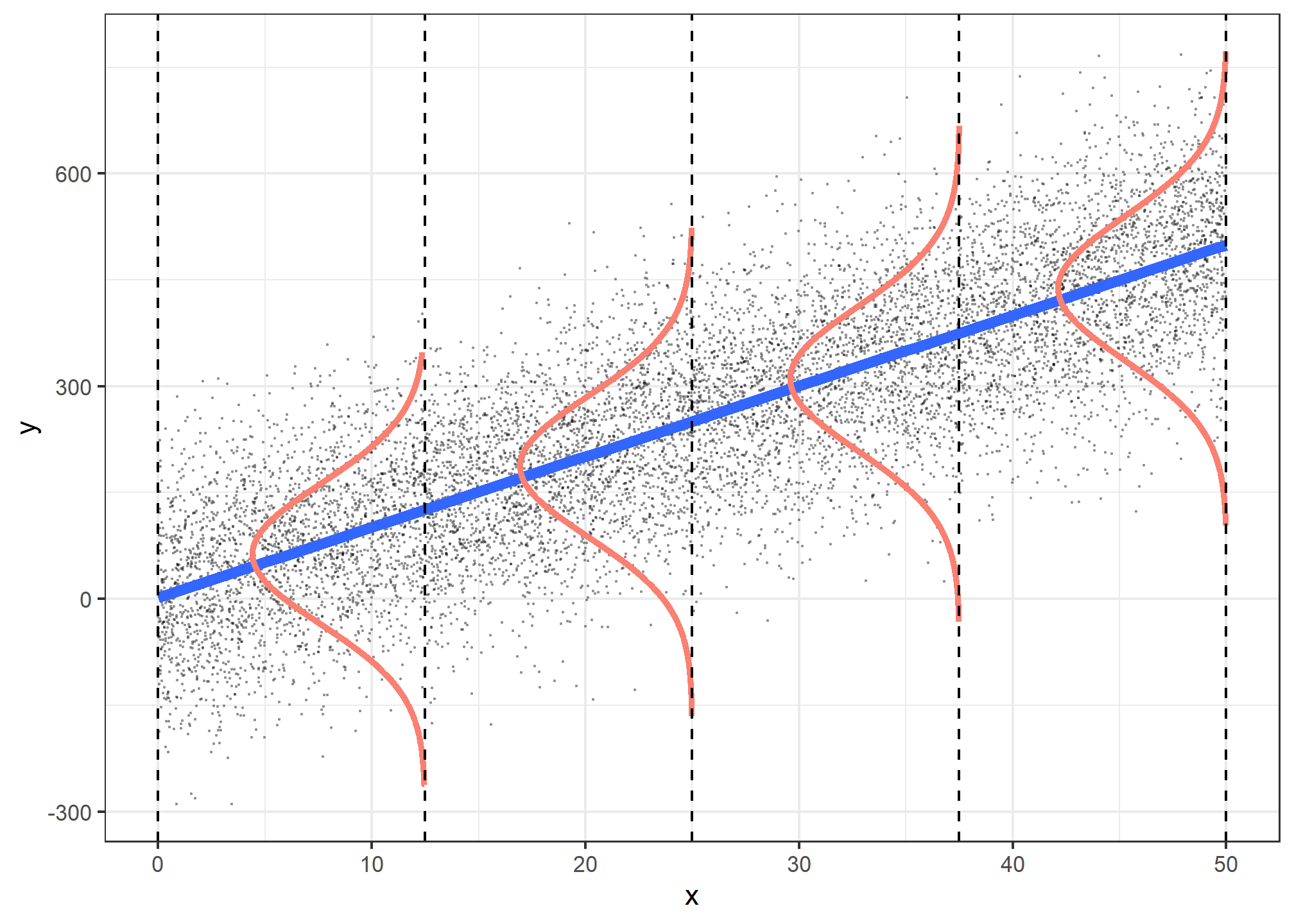
Figure 1: Assumptions for linear ordinary least squares (OLS) regression

Regression diagnostic plots with ggfortify::autoplot()

Let us see what is happening in our models. We will use the ggfortify package and its autoplot() command to get the following regression diagnostic plots:

1. Residuals vs. Fitted: checks Linearity assumption. Residuals should be random, with no pattern, and around Y = 0; if not, there is a pattern in the data that is currently unaccounted for.
2. Normal Q-Q: checks residual Normality assumption. Deviations from a straight line indicate that residuals do not follow a Normal distribution.
3. Scale-Location: checks whether residuals have equal/constant variance or not. Positive or negative trends across the fitted values indicate variability that is not constant.
4. Residuals vs. Leverage: check for influential points. Points with high leverage (having unusual values of the predictors) and/or high absolute residuals can have an undue influence on estimates of model parameters.

model1 <- lm(body_mass_g ~ flipper_length_mm, data = penguins)

model2 <- lm(body_mass_g ~ flipper_length_mm + species , data = penguins)

model3 <- lm(body_mass_g ~ flipper_length_mm + species + sex , data = penguins)

model4 <- lm(body_mass_g ~ flipper_length_mm + species + sex , data = penguins)

model5 <- lm(body_mass_g ~ flipper_length_mm + species + sex + bill_length_mm + bill_depth_mm , data = penguins)

model6 <- lm(body_mass_g ~ . , data = penguins)


library(ggfortify)

autoplot(model1) +
  theme_minimal() + 
  labs (title = "Model 1 Diagnostic Plots")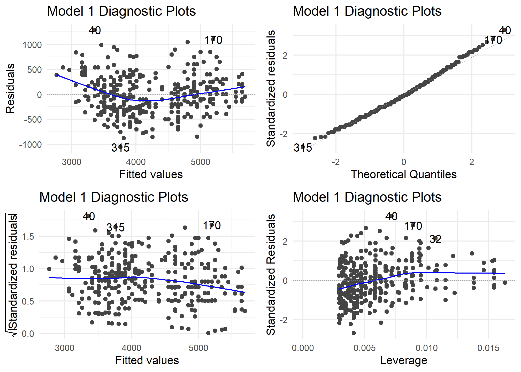

autoplot(model2) +
  theme_minimal() + 
  labs (title = "Model 2 Diagnostic Plots")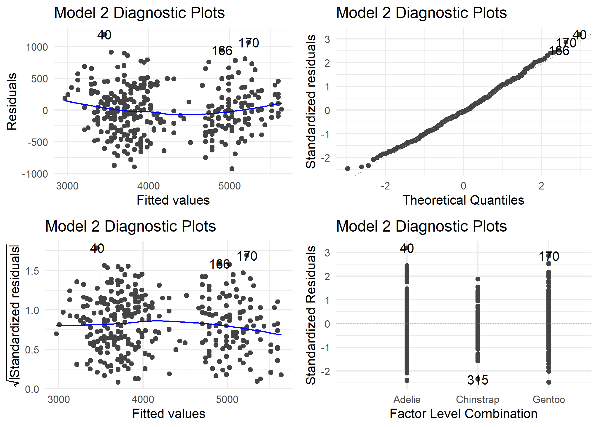

autoplot(model3) +
  theme_minimal() + 
  labs (title = "Model 3 Diagnostic Plots")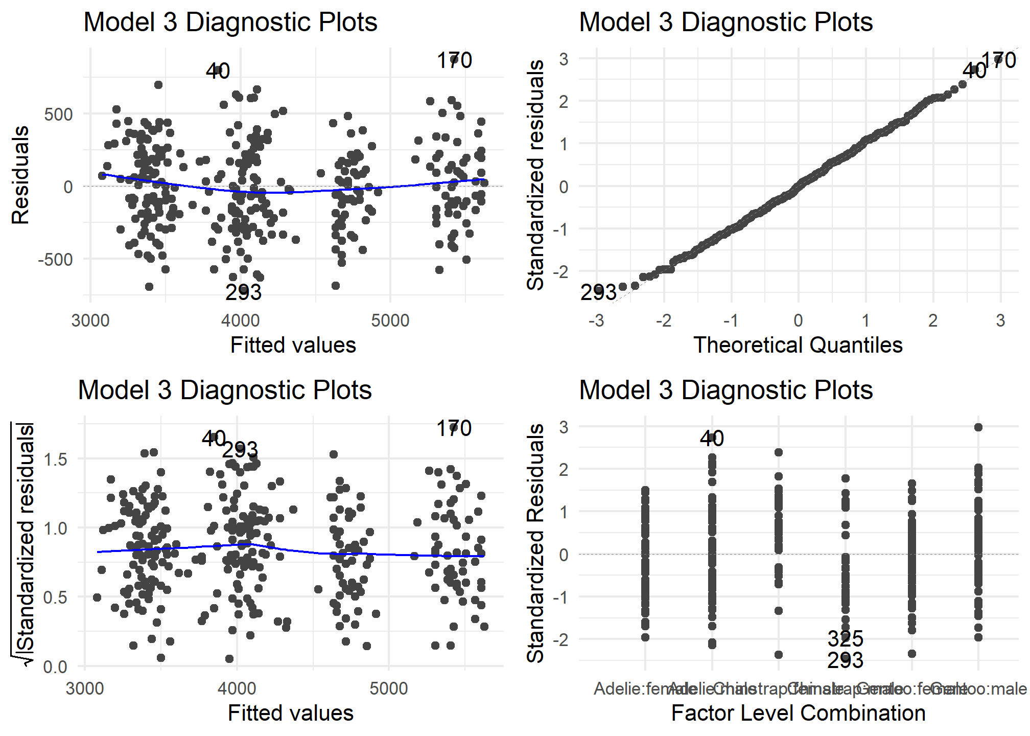

autoplot(model4) +
  theme_minimal() + 
  labs (title = "Model 4 Diagnostic Plots")

autoplot(model5) +
  theme_minimal() + 
  labs (title = "Model 5 Diagnostic Plots")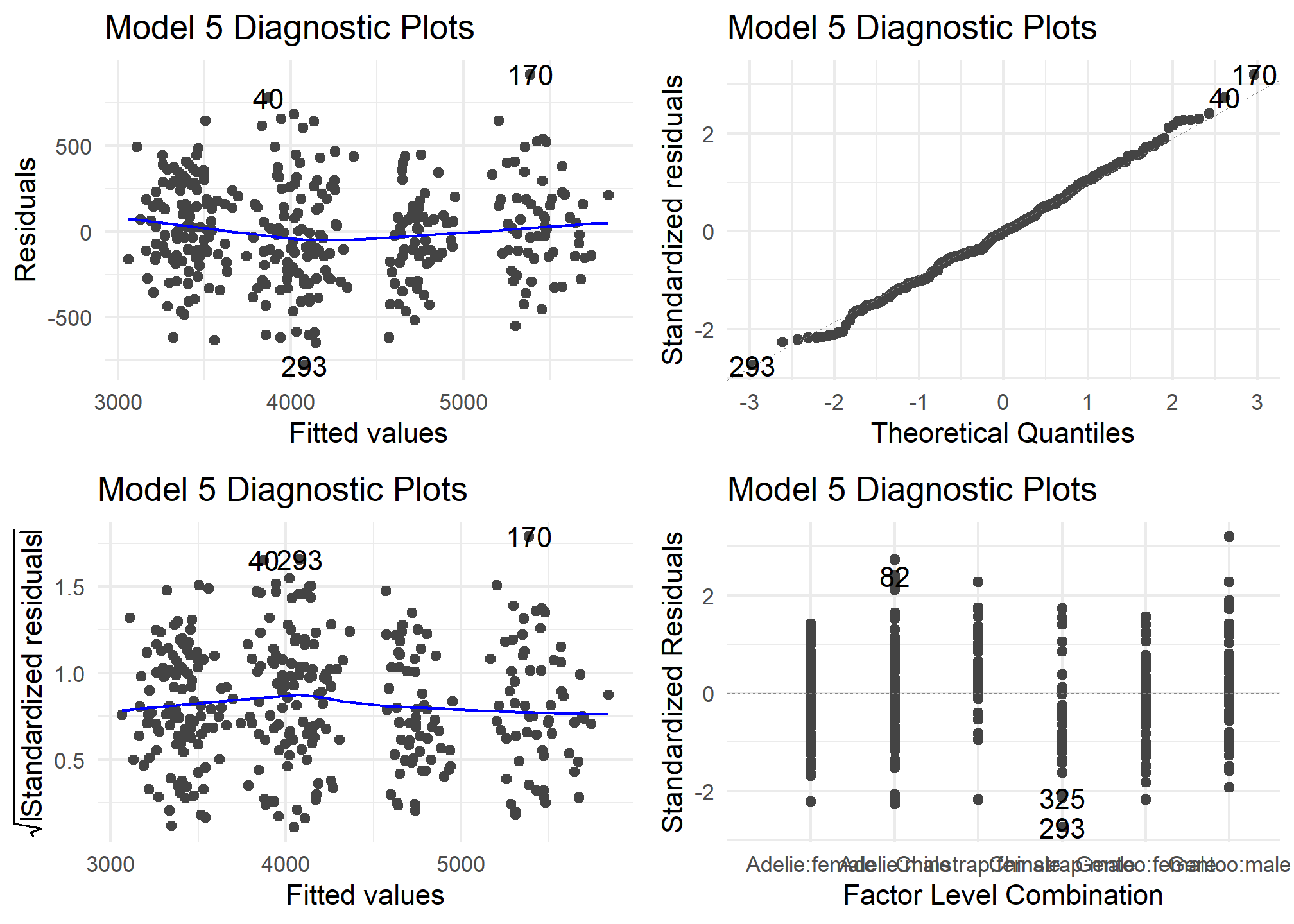

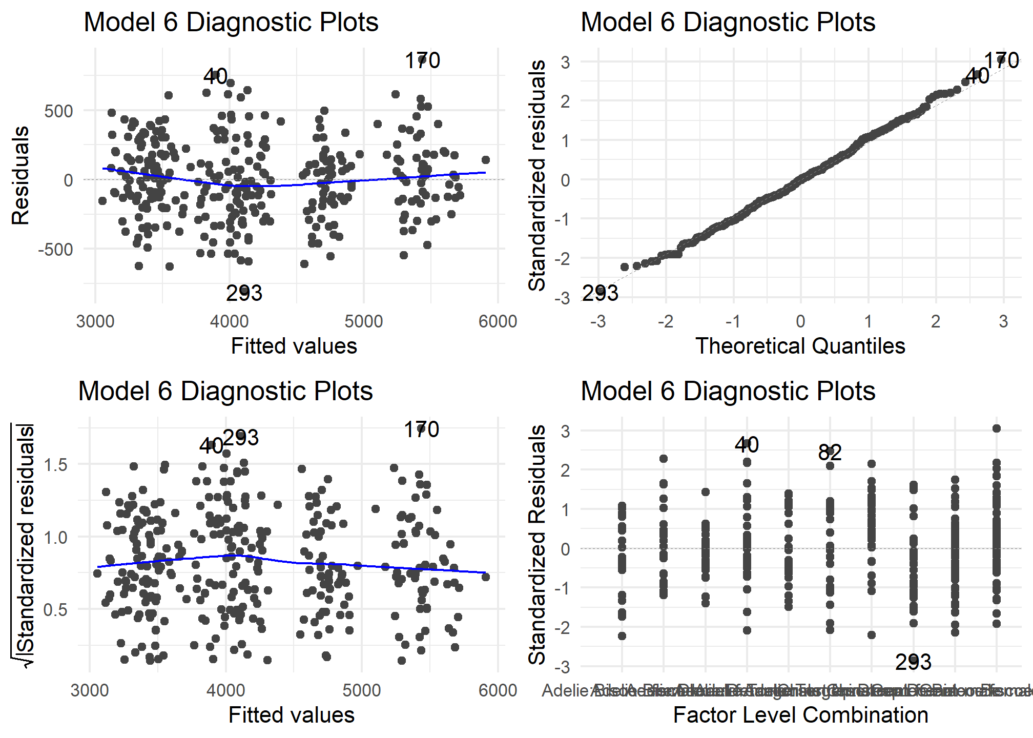
autoplot(model6) +
  theme_minimal() + 
  labs (title = "Model 6 Diagnostic Plots")