Sampling and confidence intervals (CI)
We are back to dealing with penguins, and we want to explore body mass and flipper length across the three different species.
Summary statistics
penguins %>%
  group_by(species) %>%
  summarize(across(c( body_mass_g, flipper_length_mm),
                   mean, na.rm = TRUE)) %>%
kable()| species | body_mass_g | flipper_length_mm |
|---|---|---|
| Adelie | 3701 | 190 |
| Chinstrap | 3733 | 196 |
| Gentoo | 5076 | 217 |
Boxplots
body_mass_plot <- ggplot(data = penguins, aes(y = species, x= body_mass_g)) +
  geom_boxplot(aes(color = species), width = 0.3, show.legend = FALSE) +
  geom_jitter(aes(color = species), alpha = 0.5, show.legend = FALSE, position = position_jitter(width = 0.2, seed = 0)) +
  scale_color_manual(values = c("darkorange","purple","cyan4")) +
  theme_minimal() +
  labs(title = "Penguin size, Palmer Station LTER",
       subtitle = "Body mass (in grams) for Adelie, Chinstrap and Gentoo Penguins",
       y = "Species",
       x = "Body mass (grams)")

body_mass_plot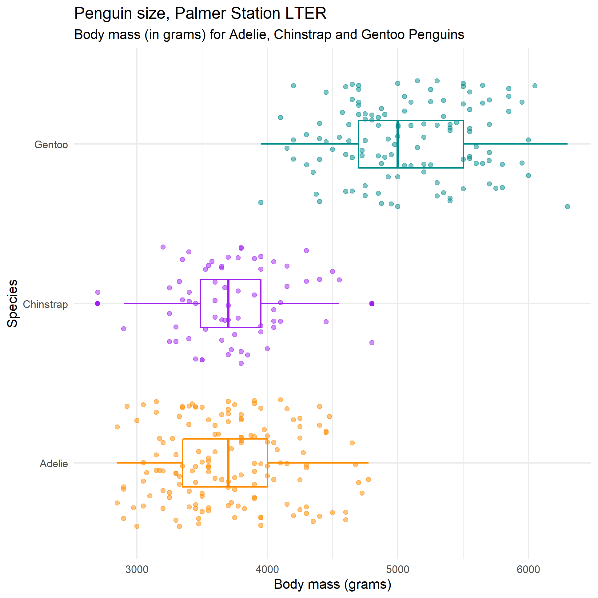
flipper_plot <- ggplot(data = penguins, aes(y = species, x = flipper_length_mm)) +
  geom_boxplot(aes(color = species), width = 0.3, show.legend = FALSE) +
  geom_jitter(aes(color = species), alpha = 0.5, show.legend = FALSE, position = position_jitter(width = 0.2, seed = 0)) +
  scale_color_manual(values = c("darkorange","purple","cyan4")) +
  theme_minimal() +
  labs(title = "Penguin size, Palmer Station LTER",
       subtitle = "Flipper length for Adelie, Chinstrap and Gentoo Penguins",
       y = "Species",
       x = "Flipper length (mm)")


flipper_plot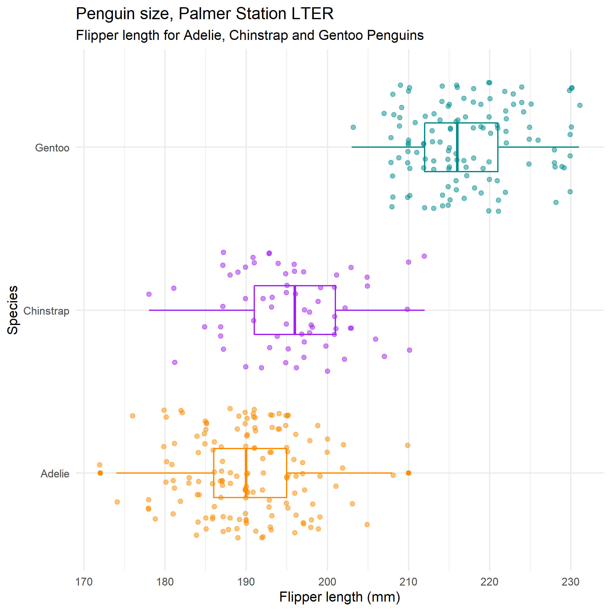
Confidence Intervals (CI)
CIs for body mass
formula_ci_body_mass <- penguins %>%
  group_by(species) %>%
  summarise( mean_body_mass = mean(body_mass_g, na.rm = TRUE),
             sd_mass = sd(body_mass_g, na.rm = TRUE),
             count = n(),

             # get t-critical value with (n-1) degrees of freedom
             t_critical = qt(0.975, count-1),
             se = sd_mass/sqrt(count),
             margin_of_error = t_critical * se,
             ci_low = mean_body_mass - margin_of_error,
             ci_high = mean_body_mass + margin_of_error
  )


formula_ci_body_mass %>%
kable()| species | mean_body_mass | sd_mass | count | t_critical | se | margin_of_error | ci_low | ci_high |
|---|---|---|---|---|---|---|---|---|
| Adelie | 3701 | 459 | 152 | 1.98 | 37.2 | 73.5 | 3627 | 3774 |
| Chinstrap | 3733 | 384 | 68 | 2.00 | 46.6 | 93.0 | 3640 | 3826 |
| Gentoo | 5076 | 504 | 124 | 1.98 | 45.3 | 89.6 | 4986 | 5166 |
#visualise  CIs for all species
ggplot(formula_ci_body_mass,
       aes(x=reorder(species, mean_body_mass),
           y=mean_body_mass,
           colour=species)) +
  geom_point() +
  scale_colour_manual(values = c("darkorange","purple","cyan4")) +
  geom_errorbar(width=.2, aes(ymin=ci_low, ymax=ci_high)) +
  labs(x=" ",
       y= "Mean body mass (grams)",
       title="Which species has the highest mean weight?") +
  theme_minimal()+
  coord_flip()+
  theme(legend.position = "none")+
  NULL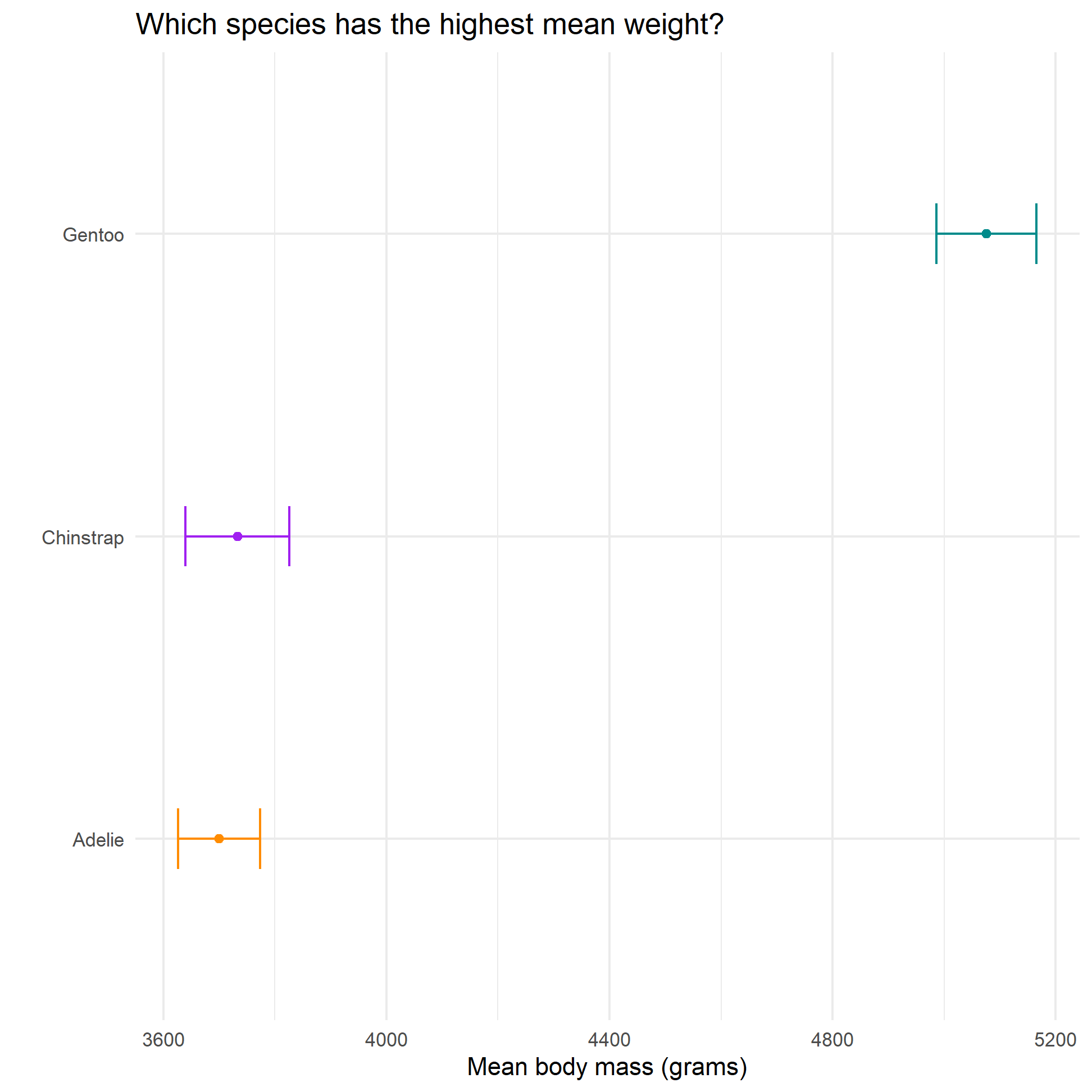
# we will draw a violin plot and then use position="jitter" or geom_jitter()
# to see how spread out the actual points are

ggplot(data = penguins, aes(y = species, x= body_mass_g)) +
  geom_violin(aes(colour = species), width = 0.3, show.legend = FALSE) +
  geom_jitter(aes(colour = species), alpha = 0.5, show.legend = FALSE, position = position_jitter(width = 0.2, seed = 0)) +
  scale_color_manual(values = c("darkorange","purple","cyan4")) +

 # superimpose  the mean as a big orange dot
  geom_point(data = formula_ci_body_mass,
             aes(x=mean_body_mass, y = species), colour = "orange", size = 8)+


  theme_minimal() +
  labs(title = "Penguin size, Palmer Station LTER",
       subtitle = "Body mass (in grams) for Adelie, Chinstrap and Gentoo Penguins",
       y = "Species",
       x = "Body mass (grams)")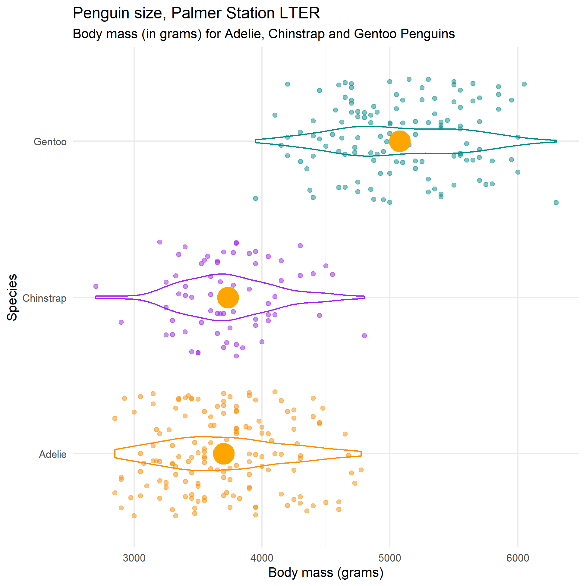
CIs for flipper length
formula_ci_flipper_length <- penguins %>%
  group_by(species) %>%
  summarise( mean_flipper_length = mean(flipper_length_mm, na.rm = TRUE),
             sd_flipper_length = sd(flipper_length_mm, na.rm = TRUE),
             count = n(),

             # get t-critical value with (n-1) degrees of freedom
             t_critical = qt(0.975, count-1),
             se = sd_flipper_length/sqrt(count),
             margin_of_error = t_critical * se,
             ci_low = mean_flipper_length - margin_of_error,
             ci_high = mean_flipper_length + margin_of_error
  )


formula_ci_flipper_length %>%
kable()| species | mean_flipper_length | sd_flipper_length | count | t_critical | se | margin_of_error | ci_low | ci_high |
|---|---|---|---|---|---|---|---|---|
| Adelie | 190 | 6.54 | 152 | 1.98 | 0.530 | 1.05 | 189 | 191 |
| Chinstrap | 196 | 7.13 | 68 | 2.00 | 0.865 | 1.73 | 194 | 198 |
| Gentoo | 217 | 6.49 | 124 | 1.98 | 0.582 | 1.15 | 216 | 218 |
#visualise  CIs for all species
ggplot(formula_ci_flipper_length,
       aes(x=reorder(species, mean_flipper_length),
           y=mean_flipper_length,
           colour=species)) +
  geom_point() +
  scale_colour_manual(values = c("darkorange","purple","cyan4")) +
  geom_errorbar(width=.2, aes(ymin=ci_low, ymax=ci_high)) +
  labs(x=" ",
       y= "Mean flipper length (mm)",
       title="Which species has the longest mean flipper?") +
  theme_minimal()+
  coord_flip()+
  theme(legend.position = "none")+
  NULL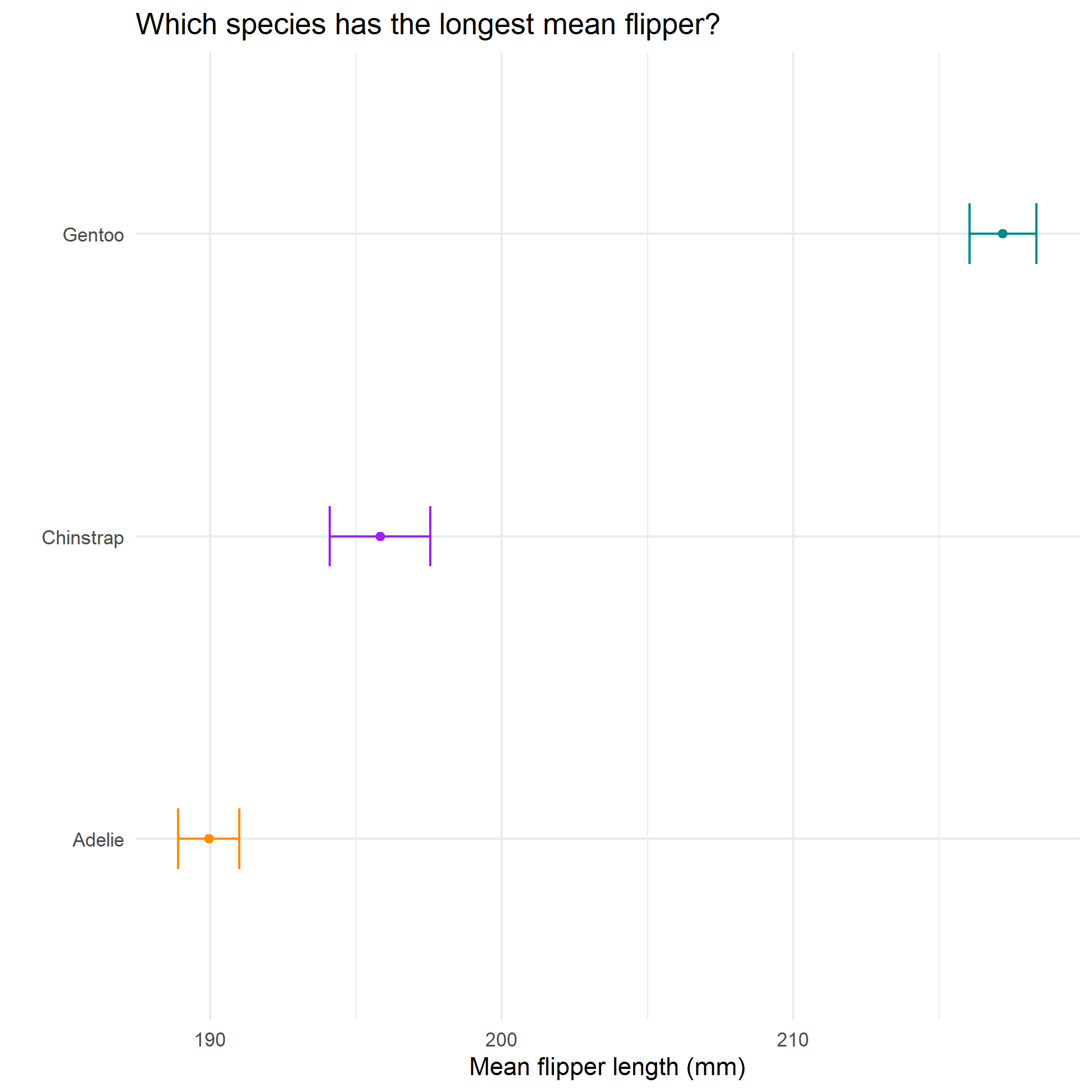
# we will draw a violin plot and then use position="jitter" or geom_jitter()
# to see how spread out the actual points are

ggplot(data = penguins, aes(y = species, x= flipper_length_mm)) +
  geom_violin(aes(colour = species), width = 0.3, show.legend = FALSE) +
  geom_jitter(aes(colour = species), alpha = 0.5, show.legend = FALSE, position = position_jitter(width = 0.2, seed = 0)) +
  scale_color_manual(values = c("darkorange","purple","cyan4")) +

 # superimpose  the mean as a big orange dot
  geom_point(data = formula_ci_flipper_length,
             aes(x=mean_flipper_length, y = species), colour = "orange", size = 8)+

  theme_minimal() +
  labs(title = "Penguin size, Palmer Station LTER",
       subtitle = "Flipper length (in mm) for Adelie, Chinstrap and Gentoo Penguins",
       y = "Species",
       x = "Flipper length (mm)")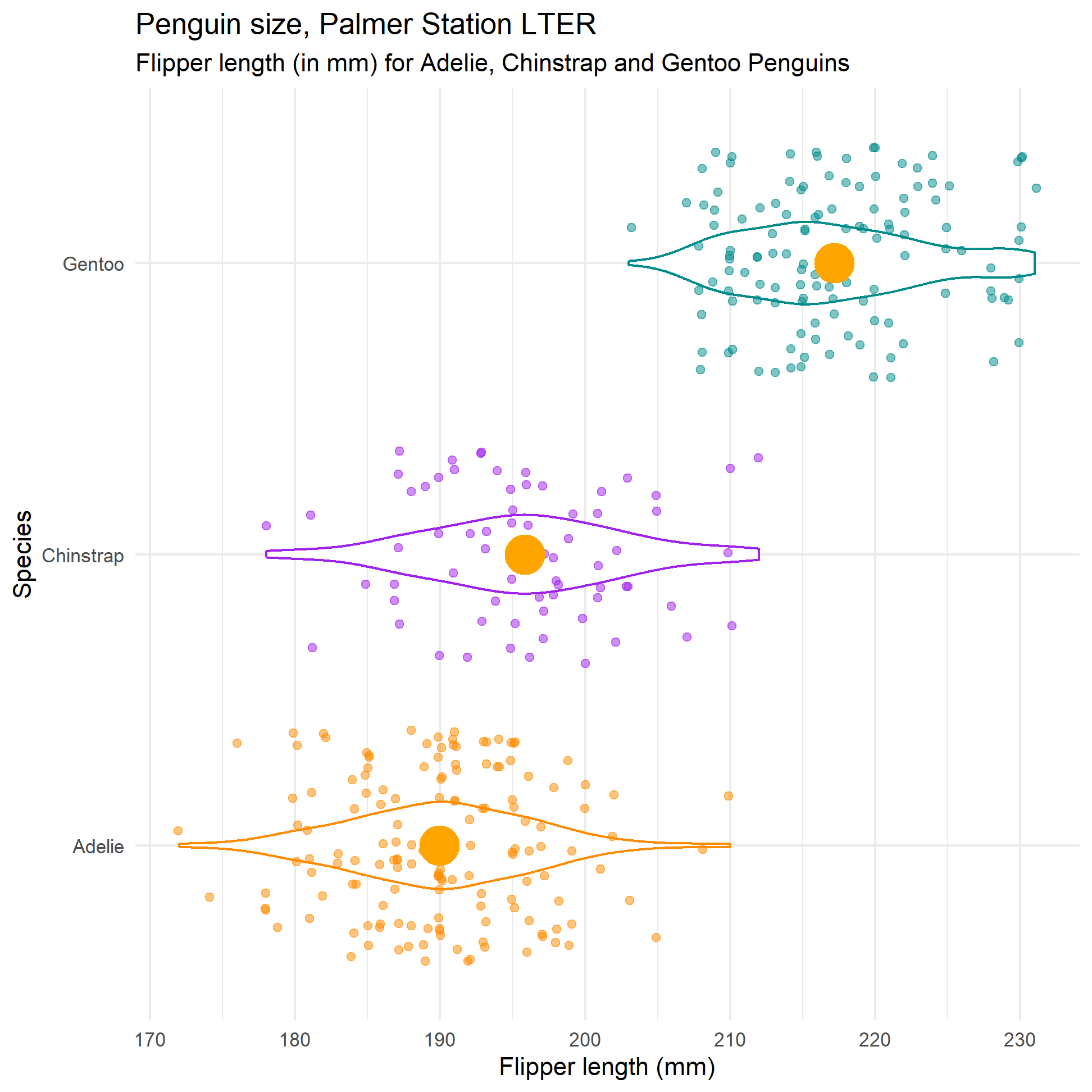
Remember in the penguins data, we saw that Gentoo penguins are very unlike the other two; however, what if we wanted to compare Adelie and Chinstrap both in terms of body mass and flipper length? By looking at the confidence intervals, we already have an indication as to whether there is a difference or not. We will use a t-Test to check if the group means are different.
Briefly, a t-Test should be used when we want to assess whether the mean between two groups are similar or not. The null hypothesis for a t-test is that the two means are equal, and the alternative is that they are not.
t-Test assuming unequal variance
R’s built-in function for running a t-test is t.test() and by default R assumes that the variance in the two groups’ populations is not equal.
t-Test for body mass
Remember that in our plots, body mass seemed to be fairly similar. While there was variability between the two species, the two average values were fairly similar and the two Confidence Intervals overlapped quite a bit.
When we run our hypothesis test, we must first set up the hypotheses.
- Null Hypothesis, \(H_0\): There is no difference in mean body mass measurements between the two species (Adelie and Chinstrap). In other words \(\mu_1 = \mu_2\), or their difference is equal to 0.
- Alternative Hypothesis, \(H_1\): There is a difference in mean body mass measurements between the two species.
Does the data provide enough evidence to reject the null hypothesis, or could the variation be due to luck? Typically, we want the p-value to be less than 5%, or equivalently the t-stat to be roughly more than 2, as fairly strong evidence to reject the null hypothesis.
#select only Adelie and Chinstrap penguins
adelie_chinstrap_test_data <- penguins %>%
  filter(species %in% c("Adelie", "Chinstrap"))


test1 <- t.test(body_mass_g ~ species,
        data = adelie_chinstrap_test_data)

test1
##
## Welch Two Sample t-test
##
## data: body_mass_g by species
## t = -0.5, df = 152, p-value = 0.6
## alternative hypothesis: true difference in means is not equal to 0
## 95 percent confidence interval:
## -150.4 85.5
## sample estimates:
## mean in group Adelie mean in group Chinstrap
## 3701 3733In our case, the t-test confirms what we already knew. First, the t-value is -0.5 and the p-value=0.6. Another way to look at it, is that the CI for the difference between the two means is [-150.4, 85.5] which contains zero indicating that we do not have strong evidence to reject the null hypothesis.
We can use broom:tidy() to convert these t-test results to a nice data frame.
test1_tidy <- tidy(test1) %>%
  # Calculate difference in means, since t.test() doesn't actually do that
  mutate(estimate = estimate1 - estimate2) %>%
  # Rearrange columns
  select(starts_with("estimate"), everything())

test1_tidy
## # A tibble: 1 x 10
## estimate estimate1 estimate2 statistic p.value parameter conf.low conf.high
## <dbl> <dbl> <dbl> <dbl> <dbl> <dbl> <dbl> <dbl>
## 1 -32.4 3701. 3733. -0.543 0.588 152. -150. 85.5
## # ... with 2 more variables: method <chr>, alternative <chr>A much cleaner output! The estimated average difference in body mass is -32.4g (we subtracted Adelie - Chinstrap, 3701-3733), the t-statistic = -0.543 and the p-value = 0.588, way greater than 0.05.
t-Test for flipper length
- Null Hypothesis, \(H_0\): There is no difference in mean flipper length measurements between the two species (Adelie and Chinstrap).
- Alternative Hypothesis, \(H_1\): There is a difference in mean flipper length measurements between the two species.
test2 <- t.test(flipper_length_mm ~ species,
        data = adelie_chinstrap_test_data)

test2_tidy <- tidy(test2) %>%
  # Calculate difference in means, since t.test() doesn't actually do that
  mutate(estimate = estimate1 - estimate2) %>%
  # Rearrange columns
  select(starts_with("estimate"), everything())

test2_tidy
## # A tibble: 1 x 10
## estimate estimate1 estimate2 statistic p.value parameter conf.low conf.high
## <dbl> <dbl> <dbl> <dbl> <dbl> <dbl> <dbl> <dbl>
## 1 -5.87 190. 196. -5.78 6.05e-8 120. -7.88 -3.86
## # ... with 2 more variables: method <chr>, alternative <chr>In our case, the t-test confirms what we already knew. the t-value is well above 2 and the p-value well below 0.05, indicating that we have strong evidence to reject the null hypothesis and therefore determine that there is a difference in mean flipper length.
The estimated average difference in flipper length is -5.9mm, the t-statistic is t-stat = -5.78 and the p-value = 6.05e-08 = \(6.05*10^{-8} = 0.00000605\), a tiny number which is way less than 0.05.
So where does this leave us?
- In terms of body mass even though we measured an average difference of 32 grams, this is not statistically significant, as its t-statistic was less than 2 and, equivalently, its p-value is >> 0.05
- In terms of flipper length, he measured average difference of 5.87mm is statistically significant as the t-statistic is 5.78 and the p-value <<< 0.0.5
t-Test assuming equal variance
We can run t.test() assuming the two groups have equal variance.
test1_equal_variance <- t.test(body_mass_g ~ species,
        data = adelie_chinstrap_test_data,
        var.equal = TRUE) # assume equal variance

test1_tidy_equal_variance <- tidy(test1_equal_variance) %>%
  # Calculate difference in means, since t.test() doesn't actually do that
  mutate(estimate = estimate1 - estimate2) %>%
  # Rearrange columns
  select(starts_with("estimate"), everything())

test1_tidy_equal_variance
## # A tibble: 1 x 10
## estimate estimate1 estimate2 statistic p.value parameter conf.low conf.high
## <dbl> <dbl> <dbl> <dbl> <dbl> <dbl> <dbl> <dbl>
## 1 -32.4 3701. 3733. -0.508 0.612 217 -158. 93.4
## # ... with 2 more variables: method <chr>, alternative <chr>test2_equal_variance <- t.test(flipper_length_mm ~ species,
data = adelie_chinstrap_test_data,
var.equal = TRUE) # assume equal variance
test2_tidy_equal_variance <- tidy(test2_equal_variance) %>%
# Calculate difference in means, since t.test() doesn't actually do that
mutate(estimate = estimate1 - estimate2) %>%
# Rearrange columns
select(starts_with("estimate"), everything())
test2_tidy_equal_variance## # A tibble: 1 x 10
## estimate estimate1 estimate2 statistic p.value parameter conf.low conf.high
## <dbl> <dbl> <dbl> <dbl> <dbl> <dbl> <dbl> <dbl>
## 1 -5.87 190. 196. -5.97 9.38e-9 217 -7.81 -3.93
## # ... with 2 more variables: method <chr>, alternative <chr>How do we test whether the two groups have equal variance?
There are several ways to check if the two groups have equal variance. For all these tests, the null hypothesis is that the two groups have equal variances.
As in all hypothesis tests, if the p-value is less than 0.05, we can assume that they have unequal variances.
Bartlett test: Check equality of variances based on the mean
body_mass_variance <- bartlett.test(body_mass_g ~ species,
        data = adelie_chinstrap_test_data)
body_mass_variance
##
## Bartlett test of homogeneity of variances
##
## data: body_mass_g by species
## Bartlett's K-squared = 3, df = 1, p-value = 0.1flipper_variance <- bartlett.test(flipper_length_mm ~ species,
data = adelie_chinstrap_test_data)
flipper_variance##
## Bartlett test of homogeneity of variances
##
## data: flipper_length_mm by species
## Bartlett's K-squared = 0.7, df = 1, p-value = 0.4In both cases, since the p-value is greater than 0.05, we cannot reject the null hypothesis so we assume that the two groups have equal variances.
Levene test Check equality of variances based on the median
Levene’s test also checks for homogeneity of variance and can based either on the mean or on the median. The median is a robust statistic, as it’s not influenced by outliers as much as the mean can be.
car::leveneTest(body_mass_g ~ species,
                center = mean,
                data = adelie_chinstrap_test_data)
## Levene's Test for Homogeneity of Variance (center = mean)
## Df F value Pr(>F)
## group 1 4.63 0.032 *
## 217
## ---
## Signif. codes: 0 '***' 0.001 '**' 0.01 '*' 0.05 '.' 0.1 ' ' 1car::leveneTest(flipper_length_mm ~ species,
center = mean,
data = adelie_chinstrap_test_data)## Levene's Test for Homogeneity of Variance (center = mean)
## Df F value Pr(>F)
## group 1 0.62 0.43
## 217car::leveneTest(body_mass_g ~ species,
center = median,
data = adelie_chinstrap_test_data)## Levene's Test for Homogeneity of Variance (center = median)
## Df F value Pr(>F)
## group 1 4.82 0.029 *
## 217
## ---
## Signif. codes: 0 '***' 0.001 '**' 0.01 '*' 0.05 '.' 0.1 ' ' 1car::leveneTest(flipper_length_mm ~ species,
center = median,
data = adelie_chinstrap_test_data)## Levene's Test for Homogeneity of Variance (center = median)
## Df F value Pr(>F)
## group 1 0.62 0.43
## 217Checking for homogeneity of variance based on the median, we can reject the null hypothesis for body mass (p-value = 0.029 < 0.05), but not for flipper length.
Fligner-Killeen test: Check homogeneity of variances based on the median, so it’s more robust to outliers
fligner.test(body_mass_g ~ species,
             data = adelie_chinstrap_test_data)
##
## Fligner-Killeen test of homogeneity of variances
##
## data: body_mass_g by species
## Fligner-Killeen:med chi-squared = 4, df = 1, p-value = 0.04fligner.test(flipper_length_mm ~ species,
data = adelie_chinstrap_test_data)##
## Fligner-Killeen test of homogeneity of variances
##
## data: flipper_length_mm by species
## Fligner-Killeen:med chi-squared = 0.5, df = 1, p-value = 0.5Let us summarise all the p-values from these tests
| Test | Body Mass | Flipper Length |
|---|---|---|
| Bartlett | 0.1 | 0.4 |
| Levene (mean) | 0.032 | 0.43 |
| Levene (median) | 0.029 | 0.43 |
| Fligner-Killeen | 0.04 | 0.4 |
In all of the Body mass tests, with the exception of the Bartlett tests, the p-value is less than 0.05. In other words, we seem to have enough evidence to conclude that the variances are different.
However, in all of the flipper length tests,, all of the p-values are > 0.0.5, which means we cannot reject the null hypothesis so we’re probably safe assuming the variances are equal and leaving var.equal = TRUE on.
Acknowledgements
- This page is adapted from the Palmer Penguins package Vignette