Import data

Overview
Importing CSV files: read_csv()
- Importing CSV files directly off the internet
- Importing CSV files saved locally
Need for speed: Enter data.table::fread() and vroom::vroom()
Other data formats
- rio: a swiss-army knife for data input-output
Never work directly on the raw data
Other links

Learning Objectives
1. Load external data from a .csv file into a data frame.
2. Describe what a data frame is.
3. Use indexing to subset specific portions of data frames.
4. Describe what a factor is.
5. Reorder and rename factors.
6. Format dates.

Overview

One of the things that I found strange when I started working with R was that, unlike other software like Excel, Stata, SPSS, etc., you couldn’t just double click on an .xls, .dta, or .sav file, load the data and look at its contents. In R, we must use a command to explicitly import the data into memory.

While there are many possible data formats, we will concentrate on CSV files, namely Comma Separated Values files that are a common way to save the raw data from spreadsheets, without any of the formatting, etc. The readr R package contains functions for importing data saved as flat file documents; readr is a core member of the tidyverse and is loaded every time you call library(tidyverse).

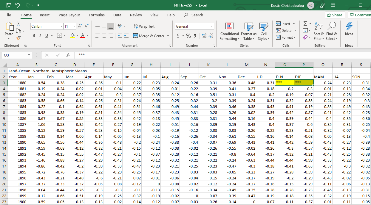
CSV file names end with a .csv and if you opened one inside Excel, it would look like a regular Excel file. NASA provides an estimate of global surface temperature change which allows us to calculate weather anomalies. The data is available at https://data.giss.nasa.gov/gistemp/tabledata_v4/NH.Ts+dSST.csv as a CSV file which you open inside Excel looks something like this:

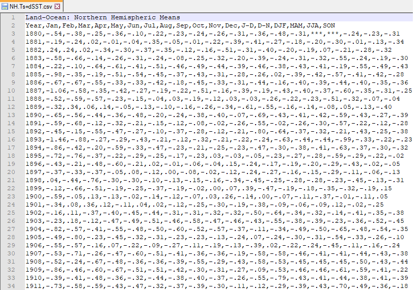
However, this is what a CSV file looks like on the inside: a bunch of values separated with commas.

By the way, if you look at the data closely, you will notice that the values in the D-N (December-November) and DJF (December-January-February) columns for the year 1880 are ***. These *** denote a missing value, in the same way that R uses the NA (or not available) value.

If you’d like R to treat these *** values as missing, you will need to convert them to NAs. One way to do this is to ask read_csv() to parse *** values as NA values when it reads in the data.

Importing CSV files: `read_csv()`

Importing CSV is part of base R using the read.csv() command. However, we will use the readr package and its read_csv() command that allows us to read flat data. read_csv() is significantly (8-10 times) faster and more user friendly than the base R command, with no need to define rownames, no stringsAsFactors = TRUE.

Even though we only concentrate on CSV files, readr has several functions that allow you to import a specific flat file format.

Function	Reads
`read_csv()`	Comma separated values
`read_csv2()`	Semi-colon separate values
`read_delim()`	General delimited files
`read_fwf()`	Fixed width files
`read_log()`	Apache log files
`read_table()`	Space separated files
`read_tsv()`	Tab delimited values

Just as you can import data, readr allows you to export data and save it locally. These functions are similar to the read_ functions and each save a tibble (or data frame) in the specific file format.

Function	Writes
`write_csv()`	Comma separated values
`write_excel_csv()`	CSV that you plan to open in Excel
`write_delim()`	General delimited files
`write_file()`	A single string, written as is
`write_lines()`	A vector of strings, one string per line
`write_tsv()`	Tab delimited values

To use a write_ function, first give it the name of the data frame to save, then give it a filename to save in your working directory.

Importing CSV files directly off the internet

If the CSV exists on the internet and you have the URL address, you don’t have to download it to your local machine and then import it; you can import it directly off the web using the URL link.

url <- "https://data.giss.nasa.gov/gistemp/tabledata_v4/NH.Ts+dSST.csv"
weather <- read_csv(url, skip = 1, na = "***")

When using the read_csv() function, we added two options:

skip = 1 option is there as the real data table only starts in Row 2, so we need to skip one row.
na = "***"option informs R how missing observations in the spreadsheet are coded. As discussed earlier, it is best to specify NA values here, as otherwise some of the data may not be recognized as numeric data.

Notice that the code above saves the output to an object named weather. You must save the output of read_csv() to an object if you wish to use it later; otherwise, read_csv() will just print the contents of the data set at the command line.

Also, the assignment statement doesn’t produce any output for weather because assignments don’t display anything. If we want to check that our data has been loaded, we can see glimpse the structure of the dataframe using glimpse() or see its contents by just typing its name: weather.

glimpse(weather) shows us the number of observations and variables, and then, for each variable, shows the variable type; in our case, all of the variables are dbl or double, namely numeric variables.
weather, just invoking the name of the dataframe, shows the contents of the dataframe in the tabular form it is saved in

glimpse(weather)

## Rows: 142
## Columns: 19
## $ Year  <dbl> 1880, 1881, 1882, 1883, 1884, 1885, 1886, 1887, 1888, 1889, 1890~
## $ Jan   <dbl> -0.36, -0.30, 0.27, -0.57, -0.17, -1.01, -0.74, -1.08, -0.48, -0~
## $ Feb   <dbl> -0.51, -0.22, 0.22, -0.66, -0.09, -0.45, -0.83, -0.70, -0.60, 0.~
## $ Mar   <dbl> -0.23, -0.04, 0.02, -0.15, -0.63, -0.24, -0.72, -0.44, -0.64, -0~
## $ Apr   <dbl> -0.30, 0.00, -0.32, -0.29, -0.60, -0.49, -0.37, -0.38, -0.22, 0.~
## $ May   <dbl> -0.06, 0.03, -0.25, -0.24, -0.36, -0.59, -0.33, -0.25, -0.16, -0~
## $ Jun   <dbl> -0.16, -0.33, -0.30, -0.12, -0.43, -0.45, -0.37, -0.20, -0.03, -~
## $ Jul   <dbl> -0.18, 0.08, -0.27, -0.03, -0.43, -0.34, -0.15, -0.24, 0.00, -0.~
## $ Aug   <dbl> -0.26, -0.04, -0.14, -0.21, -0.49, -0.41, -0.43, -0.54, -0.21, -~
## $ Sep   <dbl> -0.23, -0.27, -0.24, -0.31, -0.44, -0.40, -0.33, -0.20, -0.19, -~
## $ Oct   <dbl> -0.32, -0.44, -0.52, -0.16, -0.45, -0.37, -0.31, -0.48, -0.04, -~
## $ Nov   <dbl> -0.43, -0.37, -0.33, -0.42, -0.58, -0.39, -0.39, -0.27, -0.01, -~
## $ Dec   <dbl> -0.40, -0.23, -0.67, -0.15, -0.47, -0.12, -0.21, -0.43, -0.24, -~
## $ `J-D` <dbl> -0.29, -0.18, -0.21, -0.27, -0.43, -0.44, -0.43, -0.44, -0.23, -~
## $ `D-N` <dbl> NA, -0.19, -0.17, -0.32, -0.40, -0.47, -0.42, -0.42, -0.25, -0.1~
## $ DJF   <dbl> NA, -0.31, 0.08, -0.63, -0.13, -0.65, -0.56, -0.66, -0.51, -0.07~
## $ MAM   <dbl> -0.20, 0.00, -0.18, -0.22, -0.53, -0.44, -0.47, -0.36, -0.34, 0.~
## $ JJA   <dbl> -0.20, -0.09, -0.24, -0.12, -0.45, -0.40, -0.32, -0.33, -0.08, -~
## $ SON   <dbl> -0.33, -0.36, -0.36, -0.30, -0.49, -0.38, -0.35, -0.32, -0.08, -~

weather

## # A tibble: 142 x 19
##     Year   Jan   Feb   Mar   Apr   May   Jun   Jul   Aug   Sep   Oct   Nov   Dec
##    <dbl> <dbl> <dbl> <dbl> <dbl> <dbl> <dbl> <dbl> <dbl> <dbl> <dbl> <dbl> <dbl>
##  1  1880 -0.36 -0.51 -0.23 -0.3  -0.06 -0.16 -0.18 -0.26 -0.23 -0.32 -0.43 -0.4 
##  2  1881 -0.3  -0.22 -0.04  0     0.03 -0.33  0.08 -0.04 -0.27 -0.44 -0.37 -0.23
##  3  1882  0.27  0.22  0.02 -0.32 -0.25 -0.3  -0.27 -0.14 -0.24 -0.52 -0.33 -0.67
##  4  1883 -0.57 -0.66 -0.15 -0.29 -0.24 -0.12 -0.03 -0.21 -0.31 -0.16 -0.42 -0.15
##  5  1884 -0.17 -0.09 -0.63 -0.6  -0.36 -0.43 -0.43 -0.49 -0.44 -0.45 -0.58 -0.47
##  6  1885 -1.01 -0.45 -0.24 -0.49 -0.59 -0.45 -0.34 -0.41 -0.4  -0.37 -0.39 -0.12
##  7  1886 -0.74 -0.83 -0.72 -0.37 -0.33 -0.37 -0.15 -0.43 -0.33 -0.31 -0.39 -0.21
##  8  1887 -1.08 -0.7  -0.44 -0.38 -0.25 -0.2  -0.24 -0.54 -0.2  -0.48 -0.27 -0.43
##  9  1888 -0.48 -0.6  -0.64 -0.22 -0.16 -0.03  0    -0.21 -0.19 -0.04 -0.01 -0.24
## 10  1889 -0.27  0.3  -0.03  0.16 -0.04 -0.07 -0.08 -0.21 -0.31 -0.42 -0.62 -0.55
## # ... with 132 more rows, and 6 more variables: J-D <dbl>, D-N <dbl>,
## #   DJF <dbl>, MAM <dbl>, JJA <dbl>, SON <dbl>

When you use read_csv(), read_csv() tries to match each column of input to one of the basic data types in R. In our case, read_csv() misidentified the contents of the Year column to a real number, rather than an integer. You can correct this with R’s as.integer() function, or you can read the data in again, this time instructing read_csv() to parse the column as integers.

To do this:

add the argument col_types to read_csv()
set equal the col_types argument to a list.
add a named element to the list for each column you would like to manually parse; in our case, we want to make column ‘Year’ an integer.

weather <- read_csv(url, skip = 1, na = "***",
                   col_types = list(Year = col_integer()))

To complete the code, set Year equal to one of the functions below, each function instructs read_csv() to parse Year as a specific type of data.

Type function	Data Type
`col_character()`	character
`col_date()`	Date
`col_datetime()`	POSIXct (date-time)
`col_double()`	double (numeric)
`col_factor()`	factor
`col_guess()`	let readr guess (default)
`col_integer()`	integer
`col_logical()`	logical
`col_number()`	numbers mixed with non-number characters
`col_numeric()`	double or integer
`col_skip()`	do not read this column
`col_time()`	time

Importing CSV files saved locally

If you want to read a CSV file you have saved locally in your computer, you must let RStudio know which folder the file lives in; in more technical terms, you have to set the Working Directory. You can determine the location of your working directory by running getwd(). You can change the location of your working directory by going to Session > Set Working Directory in the RStudio IDE menu bar or use the Ctrl+Shift+H shortcut in Windows, Cmd+Shift+H in Mac to browse for the folder where the file resides.

Need for speed: Enter `data.table::fread()` and `vroom::vroom()`

If you have a file which is fairly large, the fread() function from the data.table package, data.table::fread(), and vroom::vroom() can make your life easier. You use them in a similar way to read_csv(), but they are faster.

The following table compares how long it takes to read 22.4 million rows from CDC’s COVID-19 Case Surveillance Public Use Data, with data collected as of 30 April 2021. We downloaded the CSV locally and then read it with base R read.csv(), readr::read_csv(), data.table::fread(), and vroom::vroom().

library(microbenchmark)
mbm = microbenchmark(
  baseR =   read.csv("COVID-19_Case_Surveillance_Public_Use_Data.csv"),
  readr =   read_csv("COVID-19_Case_Surveillance_Public_Use_Data.csv"),
  data.table =   fread("COVID-19_Case_Surveillance_Public_Use_Data.csv"),
  vroom =   vroom("COVID-19_Case_Surveillance_Public_Use_Data.csv"),
  times=10
)
mbm

Unit: seconds
expr	min	lq	mean	median	uq	max	neval	cld
`baseR::read.csv()`	83.24	85.60	89.71	89.01	94.26	96.95	10	d
`readr::read_csv()`	47.09	48.10	49.69	49.72	50.11	54.58	10	c
`data.table::fread()`	11.72	13.33	16.21	13.87	20.93	24.99	10	b
`vroom::vroom()`	5.71	6.01	8.28	7.738	10.99	12.49	10	a

The difference in speed is remarkable; base R is the slowest with an average loading time of about 90 seconds. read_csv() yields an average of 50 seconds, data.table:fread() reduces loading time to 16 seconds, and vroom::vroom() takes on average about 8 seconds.

Other data formats

The readr package provides efficient functions for reading and saving common flat file data formats. For other data types, consider using :

Package	Reads
readxl	Excel files (.xls, .xlsx)
haven	SPSS, Stata, and SAS files
jsonlite	json
xml2	xml
httr	web API’s
rvest	web pages (web scraping)
DBI	databases
sparklyr	data loaded into spark

`rio`: a swiss-army knife for data input-output

A really neat package to handle importing- exporting data is rio whose authors call it A Swiss-Army knife for data input-output. It works by determining the data structure from the file extension, uses reasonable defaults for data import and export (e.g., ‘stringsAsFactors=FALSE’), supports web-based import (including from SSL/HTTPS). It also has a useful function, ‘convert()’, that provides a simple method for converting between file types. You can read more about rio here

Never work directly on the raw data

In 2012 Cecilia Giménez, an 83-year-old widow and amateur painter, attempted to restore a century-old fresco of Jesus crowned with thorns in her local church in Borja, Spain. The restoration didn’t go very well, but, surprisingly, the botched restoration of Jesus fresco miraculously saved the Spanish Town.

As a most important rule, please do not work on the raw data; it’s unlikely you will have Cecilia Giménez’s good fortune to become (in)famous for your not-so-brilliant work. Make sure you import the data in R, leave the raw data aside, and if you make any changes tidying and wrangling your data, save it using write_csv() with a different file name.

Import data

Overview

Importing CSV files: read_csv()